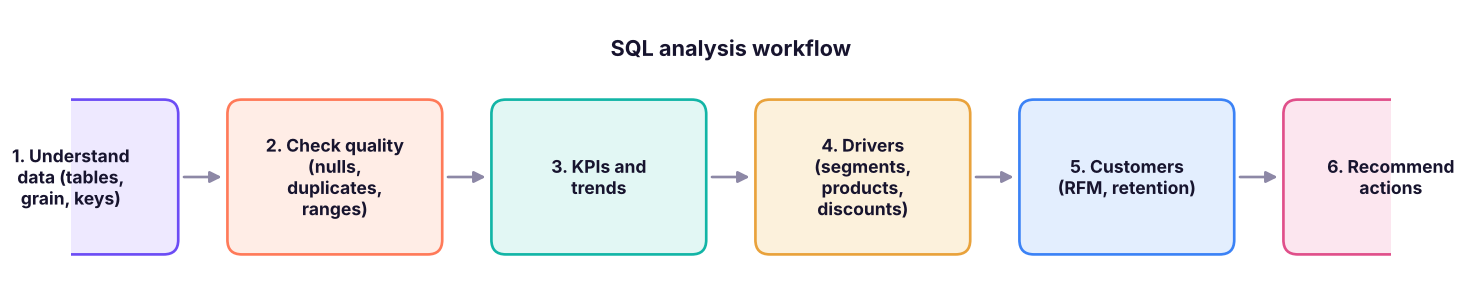
Put everything together. Work through a complete analysis of the retail business (data quality, KPIs, trends, customer segmentation, retention, product and discount analysis) using joins, CTEs and window functions, then practise 25 classic SQL interview questions with model answers.
● SQL class 5 (end-to-end case study)✦ 2026Advanced⏱ 180 min
You are the data analyst at an Indian retailer selling Furniture, Office Supplies and Technology through four regions. Sales grew from 2023 to 2025, but the CFO suspects profit is not keeping pace. Management wants answers to five questions: (1) Is the data trustworthy? (2) How are sales and profit really trending? (3) Where are we losing money and why? (4) Who are our best customers and are they staying? (5) What should we do next quarter?
A repeatable SQL analysis workflow.
Step 1: understand the data
SQL
SELECT'orders'AS tbl, COUNT(*) AS n, MIN(order_date) AS first_date, MAX(order_date) AS last_date FROM orders
UNIONALLSELECT'order_items', COUNT(*), NULL, NULLFROM order_items
UNIONALLSELECT'customers', COUNT(*), NULL, NULLFROM customers
UNIONALLSELECT'products', COUNT(*), NULL, NULLFROM products;
Result
tbl
n
first_date
last_date
orders
3200
2023-01-01
2025-12-31
order_items
6323
NULL
NULL
customers
800
NULL
NULL
products
78
NULL
NULL
4 rows × 4 columns
Grain: order_items has one row per product line in an order; orders one row per order; customers one row per customer. KPIs like "orders" must use COUNT(DISTINCT order_id), and "average order value" needs order-level totals (Lesson 10).
Step 2: data-quality checks
Always check before analysing. A compact data-quality report:
SQL
SELECT
(SELECTCOUNT(*) FROM order_items WHERE sales ISNULLOR profit ISNULLOR quantity ISNULL) AS null_measures,
(SELECTCOUNT(*) FROM order_items WHERE sales <= 0OR quantity <= 0) AS non_positive,
(SELECTCOUNT(*) FROM order_items WHERE discount < 0OR discount > 1) AS bad_discount,
(SELECTCOUNT(*) FROM orders WHERE ship_date < order_date) AS ship_before_order,
(SELECTCOUNT(*) FROM order_items oi LEFTJOIN orders o ON o.order_id = oi.order_id WHERE o.order_id ISNULL) AS orphan_items,
(SELECTCOUNT(*) FROM orders o LEFTJOIN customers c ON c.customer_id = o.customer_id WHERE c.customer_id ISNULL) AS orders_without_customer,
(SELECTCOUNT(*) - COUNT(DISTINCT item_id) FROM order_items) AS duplicate_item_ids;
Result
null_measures
non_positive
bad_discount
ship_before_order
orphan_items
orders_without_customer
duplicate_item_ids
0
0
0
0
0
0
0
1 rows × 7 columns
All zeros: the data is clean, so the numbers can be trusted. In real projects every non-zero here becomes a ticket to fix or a documented exclusion. Also check business-rule outliers:
SQL
SELECTROUND(MIN(sales), 0) AS min_sales, ROUND(MAX(sales), 0) AS max_sales,
ROUND(AVG(sales), 0) AS avg_sales,
MIN(discount) AS min_discount, MAX(discount) AS max_discount,
MIN(quantity) AS min_qty, MAX(quantity) AS max_qty
FROM order_items;
Result
min_sales
max_sales
avg_sales
min_discount
max_discount
min_qty
max_qty
42
619,290
31,854
0
0.4
1
7
1 rows × 7 columns
Step 3: KPIs and trends
SQL
WITH yearly AS (
SELECTYEAR(o.order_date) AS yr,
COUNT(DISTINCT o.order_id) AS orders,
COUNT(DISTINCT o.customer_id) AS customers,
SUM(oi.sales) AS sales,
SUM(oi.profit) AS profit
FROM orders o JOIN order_items oi ON oi.order_id = o.order_id
GROUPBYYEAR(o.order_date)
)
SELECT yr, orders, customers,
ROUND(sales, 0) AS sales,
ROUND(100.0 * (sales - LAG(sales) OVER (ORDERBY yr)) / LAG(sales) OVER (ORDERBY yr), 1) AS sales_growth_pct,
ROUND(profit, 0) AS profit,
ROUND(100.0 * (profit - LAG(profit) OVER (ORDERBY yr)) / LAG(profit) OVER (ORDERBY yr), 1) AS profit_growth_pct,
ROUND(100.0 * profit / sales, 1) AS margin_pct,
ROUND(sales / orders, 0) AS avg_order_value
FROM yearly
ORDERBY yr;
Result
yr
orders
customers
sales
sales_growth_pct
profit
profit_growth_pct
margin_pct
avg_order_value
2023
883
540
57,640,217
NULL
4,725,378
NULL
8.2
65,278
2024
1085
590
65,396,556
13.5
6,135,992
29.9
9.4
60,273
2025
1232
623
78,376,797
19.8
7,490,793
22.1
9.6
63,618
3 rows × 9 columns
Finding 1. Sales grew 13.5% in 2024 and 19.8% in 2025, and profit grew even faster (29.9% and 22.1%), so the overall margin edged up from 8.2% to 9.6%. The growth is real, but a 9.6% margin is low compared with the 17–18% earned on lines sold without a discount (you will see this in Step 4). The CFO's concern is about the quality of profit: let's look at where the money is made and lost.
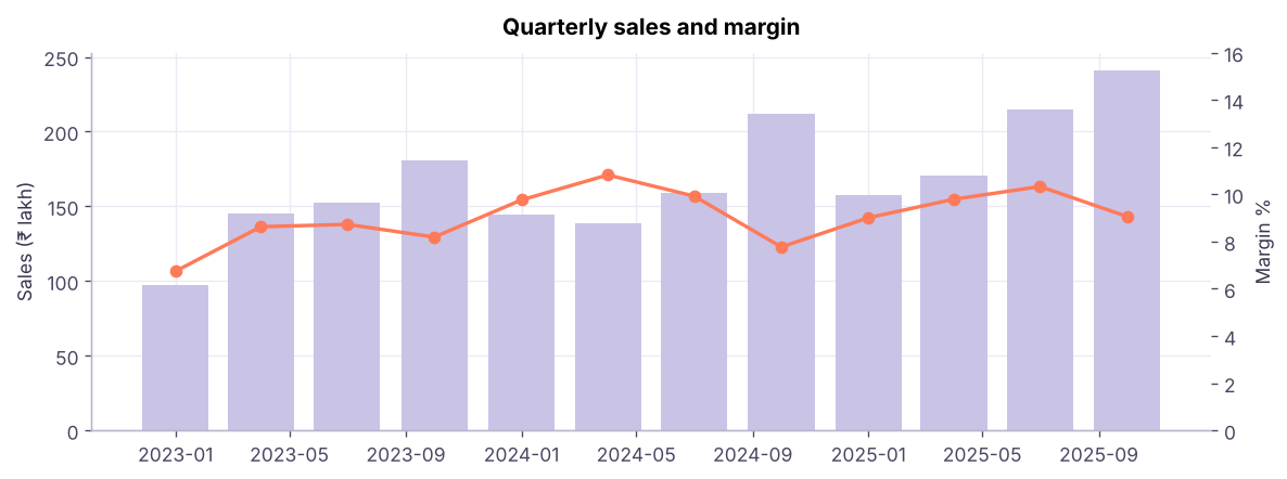
Quarterly sales and profit margin from the same data. Sales climb steadily and peak each Q4 (festive season); the margin moves in a narrow band below 12%.
Step 4: where do we lose money?
SQL
SELECT p.category, p.sub_category,
COUNT(*) AS lines,
ROUND(SUM(oi.sales), 0) AS sales,
ROUND(SUM(oi.profit), 0) AS profit,
ROUND(100.0 * SUM(oi.profit) / SUM(oi.sales), 1) AS margin_pct,
ROUND(AVG(oi.discount) * 100, 1) AS avg_discount_pct
FROM order_items oi JOIN products p ON p.product_id = oi.product_id
GROUPBY p.category, p.sub_category
ORDERBY profit;
Result
category
sub_category
lines
sales
profit
margin_pct
avg_discount_pct
Furniture
Tables
505
14,046,224
-816,042
-5.8
17.5
Furniture
Bookcases
477
11,274,849
-422,786
-3.7
18.3
Office Supplies
Art
462
245,985
36,526
14.8
7.6
Office Supplies
Binders
494
401,219
61,074
15.2
7.4
Office Supplies
Paper
559
493,232
75,040
15.2
7.2
Furniture
Furnishings
442
1,429,307
78,632
5.5
7.4
Furniture
Chairs
493
8,091,474
342,043
4.2
8.3
Technology
Accessories
445
3,178,930
369,554
11.6
7.5
Office Supplies
Storage
507
2,659,340
397,228
14.9
7.6
Office Supplies
Appliances
492
6,333,529
944,927
14.9
7.5
Technology
Phones
488
31,919,223
3,663,117
11.5
7.1
Technology
Machines
491
42,590,335
5,186,711
12.2
6.7
13 rows × 7 columns (first 12 shown)
Finding 2. Tables and Bookcases lose money, and they also carry the heaviest average discounts. Is discounting the cause? Compare margin by discount level and by whether the line is Furniture:
SQL
SELECTCASEWHEN p.category = 'Furniture'THEN'Furniture'ELSE'Other'ENDAS group_name,
CASEWHEN oi.discount = 0THEN'0%'WHEN oi.discount <= 0.2THEN'1–20%'ELSE'>20%'ENDAS discount_band,
COUNT(*) AS lines,
ROUND(SUM(oi.profit), 0) AS profit,
ROUND(100.0 * SUM(oi.profit) / SUM(oi.sales), 1) AS margin_pct
FROM order_items oi JOIN products p ON p.product_id = oi.product_id
GROUPBYCASEWHEN p.category = 'Furniture'THEN'Furniture'ELSE'Other'END,
CASEWHEN oi.discount = 0THEN'0%'WHEN oi.discount <= 0.2THEN'1–20%'ELSE'>20%'ENDORDERBY group_name, discount_band;
Result
group_name
discount_band
lines
profit
margin_pct
Furniture
0%
850
1,861,761
11.7
Furniture
1–20%
509
-317,393
-3.9
Furniture
>20%
558
-2,362,521
-21.9
Other
0%
2630
19,857,203
18.4
Other
1–20%
1434
1,014,534
2.0
Other
>20%
342
-1,701,419
-18.9
6 rows × 5 columns
Finding 3. In every group, discounts above 20% destroy margin. Furniture is hit hardest because it is discounted more often. What would profit be if lines discounted above 20% had been sold at a 20% discount instead? A rough "what-if":
SQL
WITH x AS (
SELECT oi.sales, oi.profit, oi.discount,
oi.sales / (1 - oi.discount) AS list_value,
(oi.sales / (1 - oi.discount)) * 0.8AS sales_at_20,
oi.sales - oi.profit AS cost
FROM order_items oi WHERE oi.discount > 0.2
)
SELECTCOUNT(*) AS lines_over_20pct,
ROUND(SUM(profit), 0) AS actual_profit,
ROUND(SUM(sales_at_20 - cost), 0) AS profit_if_capped_at_20pct,
ROUND(SUM(sales_at_20 - cost) - SUM(profit), 0) AS potential_gain
FROM x;
Result
lines_over_20pct
actual_profit
profit_if_capped_at_20pct
potential_gain
900
-4,063,940
-422,474
3,641,466
1 rows × 4 columns
(This ignores that a lower discount might lose some of those sales. It is an upper bound to size the opportunity, and it must be labelled as such for management.)
Step 5: customers
Top customers and concentration
SQL
WITH c AS (
SELECT o.customer_id, SUM(oi.sales) AS sales, SUM(oi.profit) AS profit, COUNT(DISTINCT o.order_id) AS orders
FROM orders o JOIN order_items oi ON oi.order_id = o.order_id
GROUPBY o.customer_id
), r AS (
SELECT *, NTILE(10) OVER (ORDERBY sales DESC) AS decile FROM c
)
SELECT decile,
COUNT(*) AS customers,
ROUND(100.0 * SUM(sales) / SUM(SUM(sales)) OVER (), 1) AS pct_of_sales,
ROUND(100.0 * SUM(profit) / SUM(SUM(profit)) OVER (), 1) AS pct_of_profit
FROM r
GROUPBY decile
ORDERBY decile;
Result
decile
customers
pct_of_sales
pct_of_profit
1
79
28.8
34.1
2
79
18.7
21.0
3
79
14.6
14.3
4
79
11.3
10.4
5
79
9.0
8.8
6
78
6.7
5.3
7
78
5.2
2.5
8
78
3.4
2.2
9
78
1.9
1.1
10
78
0.5
0.3
10 rows × 4 columns
RFM segmentation
RFM scores each customer by Recency (days since last order), Frequency (number of orders) and Monetary value (total sales). The reference date is the day after the last order in the data.
SQL
WITH base AS (
SELECT o.customer_id,
DATEDIFF(day, MAX(o.order_date), '2026-01-01') AS recency_days,
COUNT(DISTINCT o.order_id) AS frequency,
SUM(oi.sales) AS monetary
FROM orders o JOIN order_items oi ON oi.order_id = o.order_id
GROUPBY o.customer_id
), scored AS (
SELECT *,
NTILE(4) OVER (ORDERBY recency_days DESC) AS r, -- 4 = most recentNTILE(4) OVER (ORDERBY frequency) AS f,
NTILE(4) OVER (ORDERBY monetary) AS m
FROM base
)
SELECT customer_id, recency_days, frequency, ROUND(monetary, 0) AS monetary, r, f, m,
CASEWHEN r >= 3AND f >= 3AND m >= 3THEN'Champions'WHEN r >= 3AND f >= 2THEN'Loyal'WHEN r <= 2AND f >= 3AND m >= 3THEN'At risk (high value)'WHEN r = 1THEN'Lost / hibernating'ELSE'Potential'ENDAS segment
FROM scored
ORDERBY monetary DESC;
Result
customer_id
recency_days
frequency
monetary
r
f
m
segment
C0741
441
6
1,204,439
1
4
4
At risk (high value)
C0092
11
8
1,140,540
4
4
4
Champions
C0306
278
7
1,126,867
2
4
4
At risk (high value)
C0781
130
5
1,123,527
2
3
4
At risk (high value)
C0443
92
7
1,113,058
3
4
4
Champions
C0720
12
6
1,100,213
4
4
4
Champions
C0493
514
6
1,004,382
1
4
4
At risk (high value)
C0028
266
5
1,000,189
2
3
4
At risk (high value)
C0630
331
5
1,000,175
1
3
4
At risk (high value)
C0262
70
6
952,738
3
4
4
Champions
785 rows × 8 columns (first 10 shown)
SQL
WITH base AS (
SELECT o.customer_id, DATEDIFF(day, MAX(o.order_date), '2026-01-01') AS recency_days,
COUNT(DISTINCT o.order_id) AS frequency, SUM(oi.sales) AS monetary
FROM orders o JOIN order_items oi ON oi.order_id = o.order_id GROUPBY o.customer_id
), scored AS (
SELECT *, NTILE(4) OVER (ORDERBY recency_days DESC) AS r, NTILE(4) OVER (ORDERBY frequency) AS f, NTILE(4) OVER (ORDERBY monetary) AS m FROM base
), seg AS (
SELECT *, CASEWHEN r >= 3AND f >= 3AND m >= 3THEN'Champions'WHEN r >= 3AND f >= 2THEN'Loyal'WHEN r <= 2AND f >= 3AND m >= 3THEN'At risk (high value)'WHEN r = 1THEN'Lost / hibernating'ELSE'Potential'ENDAS segment FROM scored
)
SELECT segment, COUNT(*) AS customers, ROUND(SUM(monetary), 0) AS sales,
ROUND(100.0 * SUM(monetary) / SUM(SUM(monetary)) OVER (), 1) AS pct_of_sales
FROM seg GROUPBY segment ORDERBY sales DESC;
Result
segment
customers
sales
pct_of_sales
Champions
178
80,496,072
40.0
At risk (high value)
92
42,616,303
21.2
Potential
198
29,644,898
14.7
Lost / hibernating
169
24,817,833
12.3
Loyal
148
23,838,464
11.8
5 rows × 4 columns
The "At risk (high value)" group is the first win: high-spending customers who have gone quiet deserve a personal outreach before they churn. The same RFM idea is implemented with pandas in the ML track.
Retention and cohorts
A cohort groups customers by the year of their first order. Retention shows how many come back in later years.
SQL
WITH first_order AS (
SELECT customer_id, YEAR(MIN(order_date)) AS cohort_year FROM orders GROUPBY customer_id
), activity AS (
SELECTDISTINCT customer_id, YEAR(order_date) AS active_year FROM orders
)
SELECT f.cohort_year,
COUNT(DISTINCT f.customer_id) AS cohort_size,
COUNT(DISTINCTCASEWHEN a.active_year = f.cohort_year THEN a.customer_id END) AS y0,
COUNT(DISTINCTCASEWHEN a.active_year = f.cohort_year + 1THEN a.customer_id END) AS y1,
COUNT(DISTINCTCASEWHEN a.active_year = f.cohort_year + 2THEN a.customer_id END) AS y2
FROM first_order f
JOIN activity a ON a.customer_id = f.customer_id
GROUPBY f.cohort_year
ORDERBY f.cohort_year;
Result
cohort_year
cohort_size
y0
y1
y2
2023
540
540
397
415
2024
193
193
156
0
2025
52
52
0
0
3 rows × 5 columns
Divide y1 by cohort_size to get year-1 retention. About 74% of the 2023 cohort (397 of 540) ordered again in 2024, and some who skipped a year returned in 2025: this is a business with sticky customers, so reducing discounts is likely safer than the CFO fears.
Step 6: recommendations
Key takeawaysFindings and actions
Sales and profit are growing, but the margin is only 9.6%, far below the 17–18% earned on undiscounted lines.
Technology produces nearly all the profit; Furniture is net loss-making because Tables and Bookcases are sold with heavy discounts.
Discounts above 20% lose money in every category. Cap discounts at 20% (the what-if sizes the upper-bound upside at about ₹36 lakh over three years; the real gain will be lower if some customers buy less), test in two regions with an A/B design.
Customer base is sticky (strong year-on-year retention), so price discipline is lower-risk than assumed.
Re-engage "At risk (high value)" customers with a targeted offer instead of blanket discounts.
Build a monthly SQL view/dashboard with these KPIs, with data-quality checks as a first step.
SQL interview practice: 25 questions with answers
Run these on the retail database. Each answer is a runnable query.
Interview cornerQ1. Second-highest sales line.
SQL
SELECTMAX(sales) AS second_highest FROM order_items WHERE sales < (SELECTMAX(sales) FROM order_items);
Result
second_highest
551,530
1 rows × 1 columns
Interview cornerQ2. Customers with at least 8 orders.
SQL
SELECT customer_id, COUNT(*) AS orders FROM orders GROUPBY customer_id HAVINGCOUNT(*) >= 8ORDERBY orders DESC;
SELECT customer_name, COUNT(*) AS n FROM customers GROUPBY customer_name HAVINGCOUNT(*) > 1ORDERBY n DESC;
Result
customer_name
n
Sneha Joshi
6
Ananya Gupta
5
Rahul Shah
5
Asha Rao
5
Ananya Iyer
5
Saanvi Khan
5
Rohan Gupta
5
Reyansh Shah
4
Simran Khan
4
Vikram Kulkarni
4
Arjun Sharma
4
Nikhil Das
4
238 rows × 2 columns (first 12 shown)
Interview cornerQ4. Highest-selling product in each category.
SQL
WITH t AS (SELECT p.category, p.product_name, SUM(oi.sales) AS sales FROM order_items oi JOIN products p ON p.product_id = oi.product_id GROUPBY p.category, p.product_name),
r AS (SELECT *, ROW_NUMBER() OVER (PARTITIONBY category ORDERBY sales DESC) AS rn FROM t)
SELECT category, product_name, ROUND(sales, 0) AS sales FROM r WHERE rn = 1;
Result
category
product_name
sales
Furniture
Crest Table 572
3,122,680
Technology
Orbit Copier 746
16,026,341
Office Supplies
Crest Appliance 402
1,909,628
3 rows × 3 columns
Interview cornerQ5. Month-over-month growth for 2025.
SQL
WITH m AS (SELECTMONTH(order_date) AS mth, SUM(sales) AS sales FROM superstore WHEREYEAR(order_date) = 2025GROUPBYMONTH(order_date))
SELECT mth, ROUND(sales, 0) AS sales, ROUND(100.0 * (sales - LAG(sales) OVER (ORDERBY mth)) / LAG(sales) OVER (ORDERBY mth), 1) AS mom_pct FROM m ORDERBY mth;
Result
mth
sales
mom_pct
1
5,357,761
NULL
2
3,879,338
-27.6
3
6,512,645
67.9
4
6,699,805
2.9
5
6,421,274
-4.2
6
3,968,572
-38.2
7
7,190,087
81.2
8
5,802,184
-19.3
9
8,468,060
45.9
10
6,140,290
-27.5
11
10,284,516
67.5
12
7,652,267
-25.6
12 rows × 3 columns
Interview cornerQ6. Running total of sales by month in 2025.
SQL
WITH m AS (SELECTMONTH(order_date) AS mth, SUM(sales) AS sales FROM superstore WHEREYEAR(order_date) = 2025GROUPBYMONTH(order_date))
SELECT mth, ROUND(sales, 0) AS sales, ROUND(SUM(sales) OVER (ORDERBY mth ROWSBETWEENUNBOUNDEDPRECEDINGANDCURRENTROW), 0) AS running_total FROM m ORDERBY mth;
Result
mth
sales
running_total
1
5,357,761
5,357,761
2
3,879,338
9,237,099
3
6,512,645
15,749,743
4
6,699,805
22,449,548
5
6,421,274
28,870,822
6
3,968,572
32,839,394
7
7,190,087
40,029,481
8
5,802,184
45,831,665
9
8,468,060
54,299,725
10
6,140,290
60,440,015
11
10,284,516
70,724,530
12
7,652,267
78,376,797
12 rows × 3 columns
Interview cornerQ7. Customers who ordered in every year (2023, 2024 and 2025).
SQL
SELECTCOUNT(*) AS customers_all_three_years
FROM (SELECT customer_id FROM orders GROUPBY customer_id HAVINGCOUNT(DISTINCTYEAR(order_date)) = 3) AS t;
Result
customers_all_three_years
311
1 rows × 1 columns
Interview cornerQ8. Employees earning more than their department's average (HR data).
SQL
SELECTCOUNT(*) AS above_dept_avg
FROM (SELECT emp_id, monthly_income, AVG(monthly_income) OVER (PARTITIONBY department) AS avg_income FROM employees) AS t
WHERE monthly_income > avg_income;
Result
above_dept_avg
638
1 rows × 1 columns
Interview cornerQ9. Delete duplicates keeping the lowest id (pattern).
SQL
WITH d AS (SELECT *, ROW_NUMBER() OVER (PARTITIONBY customer_name, city ORDERBY customer_id) AS rn FROM dbo.customers)
DELETEFROM d WHERE rn > 1;
Interview cornerQ10. Customers with no orders in the last 6 months of 2025 but orders before that (churn candidates).
SQL
SELECTCOUNT(*) AS churn_candidates
FROM (SELECT customer_id FROM orders WHERE order_date < '2025-07-01'GROUPBY customer_id
EXCEPTSELECT customer_id FROM orders WHERE order_date >= '2025-07-01') AS t;
Result
churn_candidates
310
1 rows × 1 columns
Interview cornerQ11. Percentage of orders shipped late (more than 5 days).
SQL
SELECTROUND(100.0 * SUM(CASEWHENDATEDIFF(day, order_date, ship_date) > 5THEN1ELSE0END) / COUNT(*), 1) AS pct_late FROM orders;
Result
pct_late
31.3
1 rows × 1 columns
Interview cornerQ12. Median order-line sales.
SQL
SELECTDISTINCTPERCENTILE_CONT(0.5) WITHIN GROUP (ORDERBY sales) OVER () AS median_sales FROM order_items;
Result
median_sales
8,430
1 rows × 1 columns
Interview cornerQ13. Categories where more than 30% of lines are loss-making.
SQL
SELECT p.category, ROUND(100.0 * AVG(CASEWHEN oi.profit < 0THEN1.0ELSE0END), 1) AS pct_loss_lines
FROM order_items oi JOIN products p ON p.product_id = oi.product_id
GROUPBY p.category HAVINGAVG(CASEWHEN oi.profit < 0THEN1.0ELSE0END) > 0.3;
Result
category
pct_loss_lines
Furniture
48.9
1 rows × 2 columns
Interview cornerQ14. Cumulative percentage of sales by customer (Pareto): how many customers make 50% of sales?
SQL
WITH c AS (SELECT customer_id, SUM(sales) AS s FROM order_items oi JOIN orders o ON o.order_id = oi.order_id GROUPBY customer_id),
p AS (SELECT s, SUM(s) OVER (ORDERBY s DESCROWSBETWEENUNBOUNDEDPRECEDINGANDCURRENTROW) * 1.0 / SUM(s) OVER () AS cum FROM c)
SELECTCOUNT(*) AS customers_for_half_of_sales, (SELECTCOUNT(*) FROM c) AS total_customers FROM p WHERE cum <= 0.5;
Result
customers_for_half_of_sales
total_customers
170
785
1 rows × 2 columns
Interview cornerQ15. Swap two values in a column (pattern).
SQL
UPDATE dbo.staff SET gender = CASE gender WHEN'M'THEN'F'WHEN'F'THEN'M'ELSE gender END;
Interview cornerQ16. Find consecutive order days (streaks) for a customer: see Lesson 12 (gaps and islands).
Interview cornerQ17. Average order value per segment.
SQL
SELECT segment, ROUND(AVG(t.total), 0) AS aov
FROM (SELECT c.segment, o.order_id, SUM(oi.sales) AS total FROM orders o JOIN customers c ON c.customer_id = o.customer_id JOIN order_items oi ON oi.order_id = o.order_id GROUPBY c.segment, o.order_id) AS t
GROUPBY segment;
Result
segment
aov
Consumer
63,451
Corporate
61,899
Home Office
63,237
3 rows × 2 columns
Interview cornerQ18. Products priced above the average of their sub-category.
SQL
SELECTCOUNT(*) AS products_above_subcat_avg
FROM (SELECT product_id, list_price, AVG(list_price) OVER (PARTITIONBY sub_category) AS avg_price FROM products) AS t WHERE list_price > avg_price;
Result
products_above_subcat_avg
36
1 rows × 1 columns
Interview cornerQ19. Rows in A not in B without NOT IN trap: use NOT EXISTS (Lesson 10).
Interview cornerQ20. Pivot category sales into columns by year.
SQL
SELECT category,
ROUND(SUM(CASEWHENYEAR(order_date) = 2023THEN sales ELSE0END), 0) AS y2023,
ROUND(SUM(CASEWHENYEAR(order_date) = 2024THEN sales ELSE0END), 0) AS y2024,
ROUND(SUM(CASEWHENYEAR(order_date) = 2025THEN sales ELSE0END), 0) AS y2025
FROM superstore GROUPBY category ORDERBY category;
Result
category
y2023
y2024
y2025
Furniture
9,952,975
12,128,633
12,760,246
Office Supplies
2,611,874
3,550,109
3,971,321
Technology
45,075,369
49,717,814
61,645,230
3 rows × 4 columns
Interview cornerQ21. First and last order date and the number of days between for each customer (top 3 longest tenures).
SQL
SELECTTOP3 customer_id, MIN(order_date) AS first_order, MAX(order_date) AS last_order, DATEDIFF(day, MIN(order_date), MAX(order_date)) AS days_active
FROM orders GROUPBY customer_id ORDERBY days_active DESC;
Result
customer_id
first_order
last_order
days_active
C0079
2023-01-08
2025-12-27
1084
C0192
2023-01-24
2025-12-31
1072
C0070
2023-01-09
2025-12-13
1069
3 rows × 4 columns
Interview cornerQ22. Which month has the highest sales in each year?
SQL
WITH m AS (SELECTYEAR(order_date) AS yr, MONTH(order_date) AS mth, SUM(sales) AS sales FROM superstore GROUPBYYEAR(order_date), MONTH(order_date)),
r AS (SELECT *, RANK() OVER (PARTITIONBY yr ORDERBY sales DESC) AS rnk FROM m)
SELECT yr, mth, ROUND(sales, 0) AS sales FROM r WHERE rnk = 1ORDERBY yr;
Result
yr
mth
sales
2023
12
7,152,348
2024
11
7,284,664
2025
11
10,284,516
3 rows × 3 columns
Interview cornerQ23. How do you find the number of rows in each table of a database?
SQL
SELECT t.name AS table_name, SUM(p.rows) AS row_count
FROM sys.tables t JOIN sys.partitions p ON p.object_id = t.object_id AND p.index_id IN (0, 1)
GROUPBY t.name ORDERBY row_count DESC;
Interview cornerQ24. Explain the difference between RANK() and ROW_NUMBER() and when each is right: Lesson 11.
Interview cornerQ25. How would you explain the result of a query to a non-technical manager?
State the answer first, in one sentence with numbers ("Furniture loses ₹8.2 lakh a year, almost entirely on heavily discounted tables and bookcases"), then give the 1–2 facts that support it, the assumption or limitation, and the action you recommend.
Summary
Key takeaways
A good analysis follows a workflow: understand the grain, check data quality, calculate KPIs, find drivers, study customers, recommend actions.
Always check data quality first; label what-if estimates as estimates.
Combine CTEs, joins and window functions to build RFM segments, concentration (Pareto), cohorts and retention.
In interviews, state your assumptions, clarify the grain, write clean, formatted SQL, and explain the result in business language.
Quick quiz6 questions · tap an answer to check it
1. Why must "number of orders" use COUNT(DISTINCT order_id) when joining orders to order_items?
Answer: B. The join repeats the order for each of its items.
2. In RFM, a customer with recency 400 days, frequency 1 and low monetary value is probably:
Answer: B. Long time since the last order, few orders and low spend.
3. A cohort table shows 2023 cohort size 500, year-1 active 350. Year-1 retention is:
Answer: B. 350 ÷ 500 = 70%.
4. Which should you do before reporting KPIs?
Answer: B. Untrusted data produces untrusted numbers.
5. The what-if "profit if discounts were capped at 20%" is best described as:
Answer: C. It assumes demand would not change, so it overstates the benefit.
6. NTILE(10) over customers ordered by sales gives:
Answer: B. NTILE splits rows into n buckets.
ExerciseCapstone: your own analysis
Using only SQL on the retail database, prepare a one-page analysis answering: (1) Which three cities have the highest profit and which three the lowest? (2) What is the average days to ship by ship mode, and does a slower mode save money (profit per line)? (3) Which product's sales fell the most from 2024 to 2025? (4) Propose two actions with the numbers that support them.
Show solution
Hints: (1) GROUP BY city with ORDER BY profit ascending and descending using TOP 3 in two queries or RANK() in a CTE. (2) Join orders to order_items, AVG(DATEDIFF(day, order_date, ship_date)) and SUM(profit)/COUNT(*) by ship_mode. (3) Pivot product sales by year with conditional aggregation and compute the difference. (4) Example actions: cap Furniture discounts at 20% in two pilot regions; re-engage at-risk high-value customers. Present each action with a baseline number, an expected impact (labelled as an estimate) and a way to measure success.
Practise more online
Free, trusted places to test yourself on this topic. Links open the original site in a new tab.