
Probability and Distributions: Rules, Bayes, Binomial, Poisson and Normal
The language of uncertainty. Probability rules, conditional probability and Bayes' theorem (with a fraud-alert example), random variables and expected value, and the distributions analysts use most (Bernoulli, binomial, Poisson, uniform, normal, exponential), with scipy.stats and simulation.
- Apply the addition, multiplication and complement rules and conditional probability
- Use Bayes' theorem to update probabilities and explain base-rate effects
- Compute expected value and variance of a random variable
- Model counts and measurements with binomial, Poisson, normal and exponential distributions using scipy.stats
- Use the empirical (68-95-99.7) rule and check normality with a Q-Q plot
Probability basics
Probability is a number from 0 (impossible) to 1 (certain). For equally likely outcomes, P(event) = favourable outcomes ÷ all outcomes. In data, it is a long-run frequency.
import numpy as np, pandas as pd
from scipy import stats
rng = np.random.default_rng(7)
rolls = rng.integers(1, 7, 100_000)
print("P(six) theory 0.1667 | simulated", round((rolls == 6).mean(), 4))
print("P(even or > 4) theory", round(4 / 6, 4), "| simulated", round(((rolls % 2 == 0) | (rolls > 4)).mean(), 4))P(six) theory 0.1667 | simulated 0.1682 P(even or > 4) theory 0.6667 | simulated 0.6679
| Rule | Formula | Example |
|---|---|---|
| Complement | P(not A) = 1 − P(A) | P(no conversion) = 1 − 0.10 |
| Addition | P(A or B) = P(A) + P(B) − P(A and B) | Even or > 4: 3/6 + 2/6 − 1/6 |
| Multiplication (independent) | P(A and B) = P(A) × P(B) | Two sixes: 1/36 |
| Conditional | P(A | B) = P(A and B) ÷ P(B) | P(churn | month-to-month) |
tc = pd.DataFrame({"contract": ["M2M"] * 1690 + ["1yr"] * 739 + ["2yr"] * 571,
                   "churn": [1] * 607 + [0] * 1083 + [1] * 125 + [0] * 614 + [1] * 40 + [0] * 531})   # counts from the churn EDA
joint = pd.crosstab(tc.contract, tc.churn, normalize="all").round(3)
print(joint)
print("P(churn) =", round(tc.churn.mean(), 3), "| P(churn | M2M) =", round(tc[tc.contract == "M2M"].churn.mean(), 3), "| P(M2M | churn) =", round((tc[tc.churn == 1].contract == "M2M").mean(), 3))churn 0 1 contract 1yr 0.205 0.042 2yr 0.177 0.013 M2M 0.361 0.202 P(churn) = 0.257 | P(churn | M2M) = 0.359 | P(M2M | churn) = 0.786
P(churn | M2M) and P(M2M | churn) are different questions. Mixing them up is one of the most common reasoning errors.
Bayes' theorem
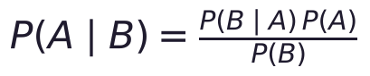
A fraud model flags 99% of fraudulent payments and wrongly flags 2% of genuine ones. Only 0.5% of payments are fraud. If a payment is flagged, how likely is it to be fraud?
p_fraud, sens, fpr = 0.005, 0.99, 0.02
p_flag = sens * p_fraud + fpr * (1 - p_fraud)                  # law of total probability
p_fraud_given_flag = sens * p_fraud / p_flag
print(f"P(flag) = {p_flag:.4f} | P(fraud | flag) = {p_fraud_given_flag:.1%}")
n = 100_000; fraud = rng.random(n) < p_fraud
flag = np.where(fraud, rng.random(n) < sens, rng.random(n) < fpr)
print(f"simulated: {fraud[flag].mean():.1%} of flagged payments are fraud ({flag.sum():,} flags, {(fraud & flag).sum()} real fraud)")P(flag) = 0.0249 | P(fraud | flag) = 19.9% simulated: 19.9% of flagged payments are fraud (2,485 flags, 495 real fraud)
Only about one flag in five is real fraud, because genuine payments vastly outnumber fraud (the base rate). This is why precision matters in imbalanced ML problems (lesson 21) and why naive Bayes classifiers work (lesson 20).
Random variables and expected value
A random variable assigns a number to each outcome. Its expected value is the probability-weighted average: the long-run mean.
values = np.array([0, 500, 2000]); probs = np.array([0.80, 0.15, 0.05])      # customer spend next month
ev = (values * probs).sum(); var = ((values - ev) ** 2 * probs).sum()
print(f"E[spend] = ₹{ev:.0f} | sd = ₹{var ** 0.5:.0f}")
cost, uplift = 60, 0.25                                                      # campaign: costs ₹60, raises spend by 25%
print(f"expected profit per customer from the campaign: ₹{ev * uplift - cost:.0f} → {'run it' if ev * uplift > cost else 'do not run it'}")E[spend] = ₹175 | sd = ₹455 expected profit per customer from the campaign: ₹-16 → do not run it
Expected value drives decisions: pricing, insurance, campaign ROI, and the "expected loss" in credit risk (PD × LGD × EAD).
Discrete distributions
| Distribution | Models | Parameters | Mean | Variance |
|---|---|---|---|---|
| Bernoulli | One yes/no trial (did this user convert?) | p | p | p(1 − p) |
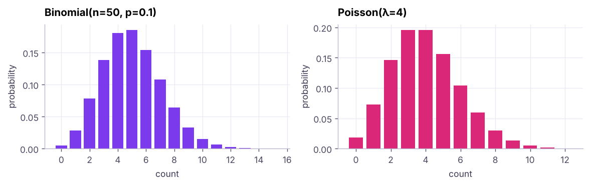
| Binomial | Number of successes in n trials | n, p | np | np(1 − p) |
| Poisson | Count of events in an interval (calls/hour, defects/batch) | λ | λ | λ |
| Geometric | Trials until first success | p | 1/p | (1 − p)/p² |
b = stats.binom(n=50, p=0.10)
print(f"P(exactly 5) = {b.pmf(5):.3f} | P(at most 2) = {b.cdf(2):.3f} | P(10 or more) = {b.sf(9):.4f} | mean {b.mean()} sd {b.std():.2f}")
po = stats.poisson(mu=4)
print(f"tickets/hour: P(0) = {po.pmf(0):.3f} | P(more than 8) = {po.sf(8):.4f} | 95th percentile = {po.ppf(0.95):.0f}")
ab = pd.read_csv("ab_test.csv"); ctrl = ab[ab.group == "A_control"]
print(f"A/B control: {ctrl.converted.sum()} conversions from {len(ctrl)} users, p̂ = {ctrl.converted.mean():.3f}")P(exactly 5) = 0.185 | P(at most 2) = 0.112 | P(10 or more) = 0.0245 | mean 5.0 sd 2.12 tickets/hour: P(0) = 0.018 | P(more than 8) = 0.0214 | 95th percentile = 8 A/B control: 198 conversions from 2000 users, p̂ = 0.099
scipy.stats methods: pmf/pdf (probability or density at a point), cdf (P(X ≤ x)), sf (P(X > x) = 1 − cdf), ppf (inverse cdf: percentiles), rvs (random samples).
Continuous distributions
For continuous variables, probability is the area under the density curve; P(X = exact value) is 0.
The normal distribution
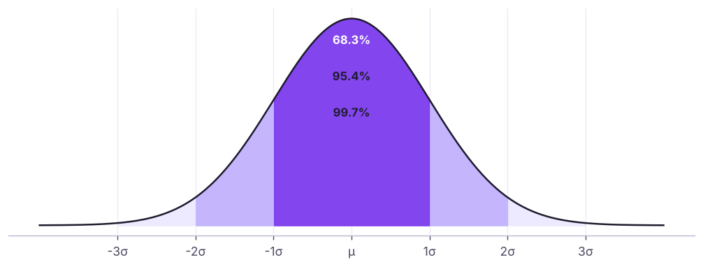
Bell-shaped, symmetric, described by mean μ and standard deviation σ. Heights, measurement errors and, crucially, sample means (next lesson) are approximately normal.
d = pd.read_csv("delivery_times.csv"); pune = d[d.city == "Pune"].delivery_minutes
mu, sd = pune.mean(), pune.std()
nd = stats.norm(mu, sd)
print(f"Pune delivery: mean {mu:.1f} min, sd {sd:.1f}")
print(f"P(late, > 40 min) model {nd.sf(40):.1%} vs data {(pune > 40).mean():.1%}")
print(f"promise time covering 95% of orders: {nd.ppf(0.95):.1f} min | within ±1 sd: {((pune - mu).abs() <= sd).mean():.0%} of orders")
print("68-95-99.7 check:", [round(float(stats.norm.cdf(k) - stats.norm.cdf(-k)), 4) for k in (1, 2, 3)], "| z for 95% two-sided:", round(stats.norm.ppf(0.975), 3))Pune delivery: mean 31.7 min, sd 6.4 P(late, > 40 min) model 9.7% vs data 13.3% promise time covering 95% of orders: 42.2 min | within ±1 sd: 68% of orders 68-95-99.7 check: [0.6827, 0.9545, 0.9973] | z for 95% two-sided: 1.96
The standard normal has μ = 0, σ = 1; any normal value converts with z = (x − μ)/σ. The number 1.96 (95% two-sided) appears in confidence intervals and tests.
Other continuous distributions
| Distribution | Models | Example |
|---|---|---|
| Uniform(a, b) | Every value equally likely | Random number generators, A/B bucket assignment |
| Exponential(λ) | Waiting time between Poisson events | Time between support calls |
| Log-normal | Positive, right-skewed values | Income, house prices, order values |
| t, χ², F | Sampling distributions for tests | t-tests, chi-square tests, ANOVA |
wait = stats.expon(scale=1 / 4)                     # 4 calls per hour → mean wait 15 minutes
print(f"P(no call for 30+ minutes) = {wait.sf(0.5):.3f} | memoryless: P(wait > 45 | already 15) = {wait.sf(0.75) / wait.sf(0.25):.3f}")P(no call for 30+ minutes) = 0.135 | memoryless: P(wait > 45 | already 15) = 0.135
Is it normal? Q-Q plots and tests
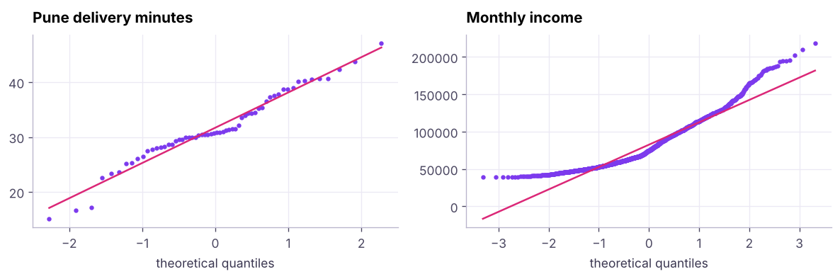
for name, data in [("delivery (Pune)", pune), ("income", hr.monthly_income), ("log income", np.log(hr.monthly_income))]:
print(f"{name:16s} Shapiro-Wilk p = {stats.shapiro(data.sample(min(len(data), 500), random_state=0)).pvalue:.4f} | skew {stats.skew(data):.2f}")delivery (Pune) Shapiro-Wilk p = 0.1629 | skew -0.15 income Shapiro-Wilk p = 0.0000 | skew 1.02 log income Shapiro-Wilk p = 0.0000 | skew 0.28
A small p-value (< 0.05) suggests the data are not normal. With large samples, tiny departures become "significant", so rely on plots and skewness too.
Summary
- Probability rules: complement, addition, multiplication (independence), conditional P(A | B) ≠ P(B | A).
- Bayes' theorem updates beliefs; low base rates make most alerts false positives.
- Expected value = probability-weighted average, the basis of ROI and risk decisions.
- Binomial (successes in n trials), Poisson (counts per interval), normal (measurements, sample means), exponential (waiting times); use
scipy.statspmf/pdf,cdf,sf,ppf,rvs. - Empirical rule 68-95-99.7; z = (x − μ)/σ; check normality with Q-Q plots and skewness.
1. A fraud test is 99% sensitive with a 2% false-positive rate, and fraud is 0.5% of payments. Roughly what share of flagged payments are fraud?
2. Which distribution models the number of support calls per hour?
3. For a binomial with n = 50 and p = 0.1, what is the mean?
4. About what share of a normal distribution lies within ±2 standard deviations?
5. Which scipy method gives P(X > x)?
6. P(churn | month-to-month) equals P(month-to-month | churn).
(1) Probability of at least one conversion from 20 visitors if p = 0.08. (2) A call centre averages 6 calls per 10 minutes; probability of more than 10 calls in 10 minutes. (3) Hyderabad delivery times: estimate P(> 45 min) with a normal model and compare with the data. (4) Simulate the Bayes fraud example with fraud at 2% instead of 0.5%. What changes?
Show solution
print(1 - 0.92 ** 20, stats.binom.sf(0, 20, 0.08))
print(stats.poisson.sf(10, 6))
hyd = d[d.city == "Hyderabad"].delivery_minutes; print(stats.norm(hyd.mean(), hyd.std()).sf(45), (hyd > 45).mean())
p_fraud = 0.02; print(sens * p_fraud / (sens * p_fraud + fpr * (1 - p_fraud))) # about 50%: the base rate mattersQ: Explain Bayes' theorem with an example. It updates a prior probability with new evidence. For a rare disease with an accurate test, a positive result can still be more likely a false positive because healthy people vastly outnumber sick ones.
Q: When would you use a Poisson distribution? For counts of independent events in a fixed time or space with a constant average rate, such as orders per minute, defects per batch or calls per hour.
Q: What is the difference between pdf and cdf? The pdf gives density at a point (probability for discrete pmf); the cdf gives the cumulative probability P(X ≤ x).
Practise more online
Free, trusted places to test yourself on this topic. Links open the original site in a new tab.