
Logistic Regression: Probabilities, Odds Ratios and Credit-Risk Scoring
Classify with probabilities. The sigmoid and log-odds, maximum likelihood and log loss, fitting logistic regression with statsmodels (inference, odds ratios) and scikit-learn (pipelines, regularisation), thresholds and decisions, multiclass logistic regression, and scoring new applicants in the Bank Loans case study.
- Explain why linear regression fails for binary targets and how the sigmoid fixes it
- Interpret coefficients as log-odds and odds ratios
- Fit, evaluate and regularise logistic regression in statsmodels and scikit-learn
- Choose a probability threshold from business costs
- Score new applicants and explain a prediction
The case: who will default?
A bank has 700 past borrowers with a known outcome (default = 1 if they failed to repay) and 150 new applicants with unknown outcomes. Features: age, education level (ed 1–5), years with current employer (employ), years at current address (address), income (thousands), debt-to-income ratio % (debtinc), credit-card debt and other debt (thousands).
import pandas as pd, numpy as np
b = pd.read_csv("bank_loans.csv")
known, new = b[b.default.notna()].copy(), b[b.default.isna()].copy()
known["default"] = known.default.astype(int)
print(len(known), "labelled |", len(new), "new applicants | default rate", round(known.default.mean(), 3))
print(known.groupby("default")[["age", "employ", "address", "income", "debtinc", "creddebt", "othdebt"]].mean().round(2))700 labelled | 150 new applicants | default rate 0.321
age employ address income debtinc creddebt othdebt
default
0 39.69 7.61 6.29 50.94 8.55 1.47 2.96
1 32.67 3.45 3.29 46.30 13.17 2.31 3.99Defaulters are younger, have shorter employment and address histories, and much higher debt-to-income ratios.
Why not linear regression?
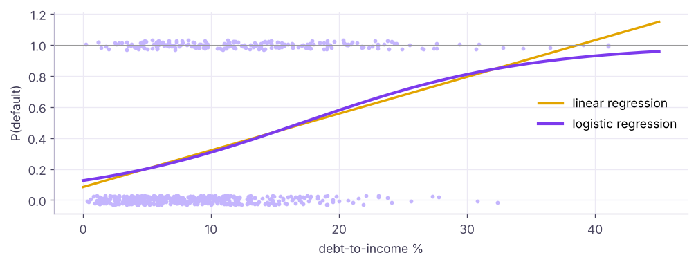
A straight line predicts values below 0 and above 1, which are not probabilities. Logistic regression passes a linear score through the sigmoid:

Equivalently, the log-odds (logit) is linear in the features:

Fitting and interpreting with statsmodels
Logistic regression is fitted by maximum likelihood: choose coefficients that make the observed outcomes most probable, equivalently minimising log loss (cross-entropy).
import statsmodels.formula.api as smf
m = smf.logit("default ~ age + ed + employ + address + income + debtinc + creddebt + othdebt", data=known).fit(disp=0)
print(m.summary2().tables[1][["Coef.", "Std.Err.", "P>|z|"]].round(4))
print(f"pseudo R² (McFadden) {m.prsquared:.3f} | log-likelihood {m.llf:.1f}")Coef. Std.Err. P>|z| Intercept -0.5739 0.5772 0.3201 age -0.0099 0.0137 0.4688 ed 0.0066 0.0989 0.9465 employ -0.1586 0.0287 0.0000 address -0.1021 0.0292 0.0005 income -0.0014 0.0084 0.8687 debtinc 0.1067 0.0330 0.0012 creddebt 0.3246 0.1227 0.0081 othdebt -0.0563 0.0579 0.3304 pseudo R² (McFadden) 0.244 | log-likelihood -332.3
odds = pd.DataFrame({"odds_ratio": np.exp(m.params), "ci_low": np.exp(m.conf_int()[0]), "ci_high": np.exp(m.conf_int()[1]), "p": m.pvalues}).drop("Intercept").round(3)
print(odds.sort_values("odds_ratio"))odds_ratio ci_low ci_high p employ 0.853 0.807 0.903 0.000 address 0.903 0.853 0.956 0.000 othdebt 0.945 0.844 1.059 0.330 age 0.990 0.964 1.017 0.469 income 0.999 0.982 1.015 0.869 ed 1.007 0.829 1.222 0.946 debtinc 1.113 1.043 1.187 0.001 creddebt 1.384 1.088 1.760 0.008
| Coefficient | Odds ratio e^β | Reading |
|---|---|---|
| β = 0 | 1 | No association |
| β > 0 | > 1 | Higher odds of default per unit |
| β < 0 | < 1 | Lower odds of default per unit |
For example, the odds ratio of about 0.85 for employ means each extra year with the current employer multiplies the odds of default by 0.85 (about 15% lower odds), holding the other variables constant. The odds ratio of about 1.38 for creddebt means each extra unit of card debt (₹1,000s) multiplies the odds by 1.38, and each extra point of debt-to-income raises the odds by about 11%. Age, education, income and other debt are not significant once the others are included.
Odds = p / (1 − p). A probability of 0.2 is odds of 0.25 ("1 to 4"). An odds ratio describes a multiplicative change in odds; the change in probability depends on where you start.
A reduced model keeps the significant predictors (a common credit-scoring practice: fewer, stable variables):
m2 = smf.logit("default ~ employ + address + debtinc + creddebt", data=known).fit(disp=0)
print(m2.params.round(3).to_dict(), "| AIC full", round(m.aic, 1), "vs reduced", round(m2.aic, 1)){'Intercept': -0.829, 'employ': -0.175, 'address': -0.113, 'debtinc': 0.099, 'creddebt': 0.25} | AIC full 682.6 vs reduced 677.0Lower AIC is better (it balances fit and complexity), so the four-variable model is preferred.
scikit-learn pipeline with regularisation
from sklearn.model_selection import train_test_split, cross_val_score
from sklearn.pipeline import make_pipeline
from sklearn.preprocessing import StandardScaler
from sklearn.metrics import roc_auc_score, accuracy_score, log_loss, classification_report
feats = ["age", "ed", "employ", "address", "income", "debtinc", "creddebt", "othdebt"]
X, y = known[feats], known.default
Xtr, Xte, ytr, yte = train_test_split(X, y, test_size=0.25, stratify=y, random_state=7)
for C in (0.01, 0.1, 1, 100):
    pipe = make_pipeline(StandardScaler(), LogisticRegression(C=C, max_iter=1000))
    cv = cross_val_score(pipe, Xtr, ytr, cv=5, scoring="roc_auc").mean()
    print(f"C = {C:<5} 5-fold ROC-AUC {cv:.3f}")
clf = make_pipeline(StandardScaler(), LogisticRegression(C=1, max_iter=1000)).fit(Xtr, ytr)
proba = clf.predict_proba(Xte)[:, 1]
print(f"\ntest: ROC-AUC {roc_auc_score(yte, proba):.3f} | accuracy {accuracy_score(yte, clf.predict(Xte)):.3f} | log loss {log_loss(yte, proba):.3f}")
print(classification_report(yte, clf.predict(Xte), target_names=["repaid", "default"], digits=3))C = 0.01 5-fold ROC-AUC 0.791
C = 0.1 5-fold ROC-AUC 0.791
C = 1 5-fold ROC-AUC 0.793
C = 100 5-fold ROC-AUC 0.792
test: ROC-AUC 0.865 | accuracy 0.817 | log loss 0.431
precision recall f1-score support
repaid 0.822 0.933 0.874 119
default 0.800 0.571 0.667 56
accuracy 0.817 175
macro avg 0.811 0.752 0.770 175
weighted avg 0.815 0.817 0.808 175C is the inverse regularisation strength (lesson 12). Standardised coefficients from the pipeline are comparable across features:
print(pd.Series(clf[-1].coef_[0], index=feats).round(3).sort_values().to_dict()){'employ': -0.875, 'address': -0.409, 'age': -0.148, 'othdebt': -0.025, 'income': -0.018, 'ed': 0.014, 'creddebt': 0.339, 'debtinc': 0.59}Choosing the threshold
predict uses a 0.5 threshold, but the right cut-off depends on costs. Suppose a missed defaulter costs the bank ₹50,000 and rejecting a good customer loses ₹10,000 of profit.
from sklearn.metrics import confusion_matrix
cost_fn, cost_fp = 50_000, 10_000
rows = []
for t in np.arange(0.1, 0.91, 0.1):
    tn, fp, fn, tp = confusion_matrix(yte, (proba >= t).astype(int)).ravel()
    rows.append({"threshold": round(t, 1), "approved": tn + fn, "defaults_caught": tp, "defaults_missed": fn, "good_rejected": fp, "cost_₹_lakh": (fn * cost_fn + fp * cost_fp) / 1e5})
th = pd.DataFrame(rows); print(th.to_string(index=False))
print("lowest-cost threshold:", th.loc[th["cost_₹_lakh"].idxmin(), "threshold"]) threshold approved defaults_caught defaults_missed good_rejected cost_₹_lakh
0.1 40 55 1 80 8.5
0.2 72 51 5 52 7.7
0.3 92 46 10 37 8.7
0.4 118 41 15 16 9.1
0.5 135 32 24 8 12.8
0.6 152 19 37 4 18.9
0.7 162 11 45 2 22.7
0.8 167 8 48 0 24.0
0.9 173 2 54 0 27.0
lowest-cost threshold: 0.2When missing a defaulter is five times as costly as rejecting a good customer, the best threshold is well below 0.5. Lesson 14 formalises this with precision, recall and ROC curves.
Scoring new applicants
final = make_pipeline(StandardScaler(), LogisticRegression(C=1, max_iter=1000)).fit(X, y)          # refit on all labelled data
new["p_default"] = final.predict_proba(new[feats])[:, 1].round(3)
best_t = th.loc[th["cost_₹_lakh"].idxmin(), "threshold"]
new["decision"] = np.where(new.p_default >= best_t, "decline / review", "approve")
print(new.decision.value_counts().to_dict())
print(new.sort_values("p_default", ascending=False)[["customer_id", "age", "employ", "debtinc", "creddebt", "p_default", "decision"]].head(5).to_string(index=False)){'decline / review': 84, 'approve': 66}
customer_id age employ debtinc creddebt p_default decision
L0782 36 0 32.9 4.73 0.961 decline / review
L0774 42 8 39.1 7.26 0.932 decline / review
L0736 32 5 28.8 7.60 0.898 decline / review
L0702 41 6 27.9 4.55 0.883 decline / review
L0753 36 6 29.7 6.09 0.876 decline / reviewExplaining one decision
one = new.sort_values("p_default", ascending=False).iloc[0]
z = (one[feats].astype(float) - final[0].mean_) / final[0].scale_
contrib = pd.Series(z.values * final[-1].coef_[0], index=feats).sort_values(ascending=False)
print(f"{one.customer_id}: P(default) {one.p_default:.2f}; log-odds contributions:", contrib.round(2).to_dict())L0782: P(default) 0.96; log-odds contributions: {'debtinc': 2.37, 'employ': 0.97, 'creddebt': 0.96, 'address': 0.13, 'income': 0.03, 'age': 0.02, 'ed': -0.01, 'othdebt': -0.17}Each contribution is a coefficient × the applicant's standardised value: positive values push towards default. This additive explanation is a big reason banks like logistic regression (and regulators require explanations of adverse decisions).
Multiclass logistic regression
With more than two classes, scikit-learn fits a multinomial (softmax) model automatically: one score per class, converted to probabilities that sum to 1.
from sklearn.datasets import load_iris
iris = load_iris(as_frame=True)
mc = make_pipeline(StandardScaler(), LogisticRegression(max_iter=1000)).fit(iris.data, iris.target)
print(mc.predict_proba(iris.data.iloc[[0, 60, 120]]).round(3), "| classes:", iris.target_names.tolist())[[0.985 0.015 0. ] [0.022 0.962 0.016] [0. 0.023 0.977]] | classes: ['setosa', 'versicolor', 'virginica']
Summary
- Logistic regression models log-odds as linear in the features and maps them to probabilities with the sigmoid; it is fitted by maximum likelihood (log loss).
- e^β is an odds ratio: > 1 raises, < 1 lowers the odds per unit, holding other features constant.
- statsmodels gives inference (p-values, CIs, AIC); scikit-learn gives pipelines, regularisation (C) and deployment.
- Choose the probability threshold from business costs, not by default 0.5.
- Coefficient × standardised value gives a transparent explanation of each prediction.
1. What does the sigmoid function do?
2. An odds ratio of 1.38 for card debt means…
3. Which loss does logistic regression minimise?
4. Missing a defaulter costs 5× more than rejecting a good customer. The best threshold is probably…
5. In scikit-learn, LogisticRegression(C=0.01) means…
6. Why do banks favour logistic regression for credit scoring?
(1) Fit a logistic regression for HR attrition with overtime, job_satisfaction, years_at_company and monthly_income. Report odds ratios. (2) What is the predicted probability for an employee with overtime, satisfaction 1, 1 year at the company and ₹50,000 income? (3) Find the threshold that maximises F1 on a validation split.
Show solution
hr = pd.read_csv("hr_employees.csv"); hr["left"] = (hr.attrition == "Yes").astype(int)
ma = smf.logit("left ~ C(overtime) + job_satisfaction + years_at_company + I(monthly_income / 10000)", data=hr).fit(disp=0)
print(np.exp(ma.params).round(3))
print(ma.predict(pd.DataFrame({"overtime": ["Yes"], "job_satisfaction": [1], "years_at_company": [1], "monthly_income": [50000]})))
from sklearn.metrics import f1_score
ts = np.linspace(.05, .95, 19); print(max(ts, key=lambda t: f1_score(yte, proba >= t)))Q: Why is it called regression if it classifies? It regresses the log-odds on the features; classification happens when you apply a threshold to the predicted probability.
Q: How do you interpret a logistic regression coefficient? A one-unit increase in the feature changes the log-odds by β, i.e. multiplies the odds by e^β, holding other features constant.
Q: What are the assumptions of logistic regression? Independent observations, a linear relationship between features and log-odds, little multicollinearity, no extreme outliers, and enough events per variable.
Practise more online
Free, trusted places to test yourself on this topic. Links open the original site in a new tab.