
Neural Networks and Deep Learning: From a Neuron to Transformers
Understand the models behind modern AI. Neurons, weights and activation functions, forward pass and backpropagation, a two-layer network written from scratch in NumPy, multilayer perceptrons in scikit-learn on images and tabular data, training practice (learning rate, batches, epochs, early stopping, dropout), and a map of CNNs, RNNs, transformers and LLMs with PyTorch and Keras code.
- Explain a neuron, layers, activation functions and the forward pass
- Explain loss, gradients and backpropagation, and train a small network from scratch
- Train and tune MLPs with scikit-learn and compare them with classical models
- Apply practical training techniques: scaling, learning rate, batching, early stopping, regularisation
- Describe CNNs, RNNs and transformers and where each is used
A neuron
An artificial neuron computes a weighted sum of its inputs plus a bias, then applies an activation function:
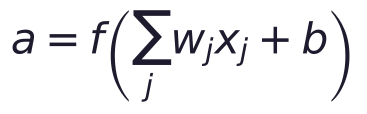
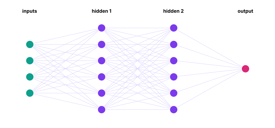
With the sigmoid activation, one neuron is logistic regression. Stacking neurons in layers lets the network learn non-linear patterns.
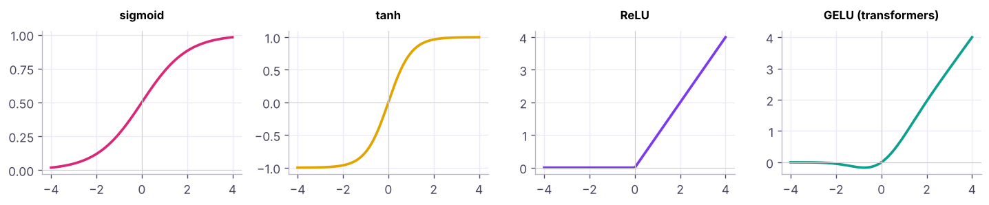
Activation functions
| Activation | Where | Why |
|---|---|---|
| ReLU (max(0, z)) | Hidden layers | Simple, fast, avoids vanishing gradients |
| GELU, SiLU | Hidden layers of transformers | Smooth variants of ReLU |
| Sigmoid | Binary output | Probability between 0 and 1 |
| Softmax | Multiclass output | Probabilities that sum to 1 |
| None (linear) | Regression output | Any real value |
Without non-linear activations, any stack of layers collapses into a single linear model.
How networks learn: backpropagation
- Forward pass: compute predictions layer by layer.
- Loss: measure the error (cross-entropy for classification, MSE for regression).
- Backward pass: use the chain rule to compute the gradient of the loss with respect to every weight (backpropagation).
- Update: gradient descent step on every weight (lesson 11), usually with the Adam optimiser on mini-batches.
- Repeat for many epochs (passes over the data).
A network from scratch
from sklearn.datasets import make_moons
X, y = make_moons(600, noise=0.2, random_state=0); y = y.reshape(-1, 1)
rng = np.random.default_rng(0)
W1, b1 = rng.normal(0, 1, (2, 16)) * np.sqrt(2 / 2), np.zeros((1, 16))          # He initialisation
W2, b2 = rng.normal(0, 1, (16, 1)) * np.sqrt(2 / 16), np.zeros((1, 1))
sigmoid = lambda z: 1 / (1 + np.exp(-z))
lr, losses = 0.5, []
for epoch in range(2000):
    z1 = X @ W1 + b1; a1 = np.maximum(0, z1)                    # forward: hidden layer (ReLU)
    p = sigmoid(a1 @ W2 + b2)                                    # forward: output (sigmoid)
    loss = -np.mean(y * np.log(p + 1e-9) + (1 - y) * np.log(1 - p + 1e-9)); losses.append(loss)
    dz2 = (p - y) / len(X)                                       # backward: output gradient
    dW2, db2 = a1.T @ dz2, dz2.sum(0, keepdims=True)
    dz1 = (dz2 @ W2.T) * (z1 > 0)                                # chain rule through ReLU
    dW1, db1 = X.T @ dz1, dz1.sum(0, keepdims=True)
    W1 -= lr * dW1; b1 -= lr * db1; W2 -= lr * dW2; b2 -= lr * db2
acc = ((p > 0.5) == y).mean()
print(f"loss: epoch 0 {losses[0]:.3f} → epoch 200 {losses[200]:.3f} → epoch 2000 {losses[-1]:.3f} | training accuracy {acc:.3f}")
print("parameters:", W1.size + b1.size + W2.size + b2.size)loss: epoch 0 0.719 → epoch 200 0.196 → epoch 2000 0.063 | training accuracy 0.977 parameters: 65
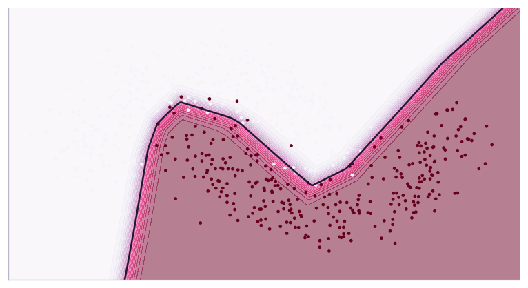
These 30 lines are the core of every deep-learning library; frameworks add automatic differentiation, GPUs, better optimisers and building blocks.
MLPs in scikit-learn
from sklearn.neural_network import MLPClassifier
from sklearn.datasets import load_digits
from sklearn.model_selection import train_test_split, cross_val_score
from sklearn.pipeline import make_pipeline
from sklearn.preprocessing import StandardScaler
from sklearn.linear_model import LogisticRegression
digits = load_digits()
Xa, Xb, ya, yb = train_test_split(digits.data, digits.target, test_size=0.3, stratify=digits.target, random_state=0)
for name, m in [("logistic regression", make_pipeline(StandardScaler(), LogisticRegression(max_iter=3000))),
                ("MLP (64)", make_pipeline(StandardScaler(), MLPClassifier((64,), max_iter=500, random_state=0))),
                ("MLP (128, 64), early stopping", make_pipeline(StandardScaler(), MLPClassifier((128, 64), alpha=1e-3, early_stopping=True, max_iter=500, random_state=0)))]:
m.fit(Xa, ya); print(f"{name:32s} test accuracy {m.score(Xb, yb):.3f}")logistic regression test accuracy 0.972 MLP (64) test accuracy 0.974 MLP (128, 64), early stopping test accuracy 0.974
import pandas as pd
from sklearn.compose import ColumnTransformer
from sklearn.preprocessing import OneHotEncoder
from sklearn.ensemble import HistGradientBoostingClassifier
tc = pd.read_csv("telecom_churn.csv"); Xc = tc.drop(columns=["customer_id", "churn", "total_charges"]); yc = (tc.churn == "Yes").astype(int)
pre = ColumnTransformer([("n", StandardScaler(), ["senior_citizen", "tenure_months", "monthly_charges", "support_calls"]), ("c", OneHotEncoder(), ["contract", "internet_service", "payment_method"])])
for name, est in [("logistic regression", LogisticRegression(max_iter=2000)), ("MLP (32, 16)", MLPClassifier((32, 16), alpha=1e-2, early_stopping=True, max_iter=1000, random_state=0)),
                  ("gradient boosting", HistGradientBoostingClassifier(max_iter=200, learning_rate=0.05, random_state=0))]:
s = cross_val_score(make_pipeline(pre, est), Xc, yc, cv=5, scoring="roc_auc"); print(f"churn {name:20s} AUC {s.mean():.3f}")churn logistic regression AUC 0.815 churn MLP (32, 16) AUC 0.802 churn gradient boosting AUC 0.782
Neural networks win on unstructured data (images, text, audio). On small tabular data, logistic regression and gradient boosting usually match or beat them with less tuning.
Training practice
| Technique | Purpose |
|---|---|
| Scale inputs | Stable, fast optimisation |
| Learning rate (and schedules) | The single most important setting |
| Mini-batches (32–512) | Efficient GPU use, regularising noise |
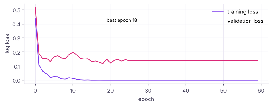
| Epochs + early stopping | Stop when validation loss stops improving |
| Dropout | Randomly switch off neurons in training: reduces overfitting |
| Weight decay (L2) | Penalise large weights (alpha in scikit-learn) |
| Batch / layer normalisation | Stabilise activations, allow higher learning rates |
| Data augmentation | Flip/crop images, paraphrase text: more data for free |
| Transfer learning | Start from a pre-trained model and fine-tune: the default today |
Deep-learning architectures
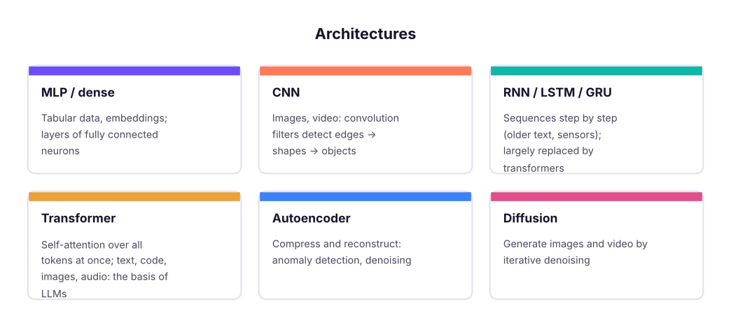
Transformers (Vaswani et al., 2017, "Attention Is All You Need") let every token look at every other token through self-attention, train in parallel on GPUs and scale to billions of parameters. Pre-trained on huge text corpora to predict the next token, then instruction-tuned and aligned with human feedback, they became large language models (GenAI track).
PyTorch and Keras
# PyTorch (pip install torch): the research and industry standard
import torch, torch.nn as nn
model = nn.Sequential(nn.Linear(64, 128), nn.ReLU(), nn.Dropout(0.2), nn.Linear(128, 10))
opt = torch.optim.AdamW(model.parameters(), lr=1e-3, weight_decay=1e-4)
loss_fn = nn.CrossEntropyLoss()
for epoch in range(20):
    for xb, yb in train_loader:                 # mini-batches
        opt.zero_grad()
        loss = loss_fn(model(xb), yb)
        loss.backward()                          # backpropagation (autograd)
opt.step() # Adam update# Keras 3 (pip install keras): high-level API on TensorFlow, JAX or PyTorch
import keras
model = keras.Sequential([keras.layers.Dense(128, activation="relu"), keras.layers.Dropout(0.2), keras.layers.Dense(10, activation="softmax")])
model.compile(optimizer="adam", loss="sparse_categorical_crossentropy", metrics=["accuracy"])
model.fit(X_train, y_train, validation_split=0.2, epochs=50, callbacks=[keras.callbacks.EarlyStopping(patience=5, restore_best_weights=True)])# Transfer learning with Hugging Face (pip install transformers): fine-tune a pre-trained model for sentiment
from transformers import pipeline
clf = pipeline("sentiment-analysis", model="distilbert-base-uncased-finetuned-sst-2-english")
clf(["Battery barely lasts half a day", "Display is bright and sharp"])Free GPUs for practice: Google Colab and Kaggle notebooks.
Summary
- A neuron = weighted sum + activation; layers of neurons with non-linear activations learn complex functions.
- Training = forward pass, loss, backpropagation (chain rule), gradient-descent updates (Adam) over epochs and mini-batches.
- Use ReLU/GELU in hidden layers, sigmoid/softmax outputs for classification; scale inputs; regularise with early stopping, dropout and weight decay.
- Neural networks excel on images, text and audio; on small tabular data, gradient boosting and logistic regression are strong competitors.
- CNNs for images, transformers for sequences and language (LLMs); PyTorch, Keras and Hugging Face are the main tools; transfer learning is the default.
1. What happens without non-linear activation functions?
2. What does backpropagation compute?
3. Which output activation for a 10-class problem?
4. Validation loss starts rising while training loss keeps falling. What is happening?
5. Which architecture is the basis of LLMs?
6. For a 2,000-row tabular churn dataset, which is usually a strong first choice?
(1) Change the hidden layer size of the NumPy network to 4 and 64: how do loss and boundary change? (2) Train an MLPRegressor on house prices and compare MAE with gradient boosting. (3) In Colab, train the PyTorch model above on the digits data.
Show solution
from sklearn.neural_network import MLPRegressor
from sklearn.ensemble import HistGradientBoostingRegressor
from sklearn.metrics import mean_absolute_error
h = pd.read_csv("house_prices.csv").dropna(subset=["area_sqft"]); h = h[h.price_lakh.between(5, 300)]
Xh = pd.get_dummies(h.drop(columns=["house_id", "price_lakh"]), drop_first=True).astype(float)
a, b, c, d = train_test_split(Xh, h.price_lakh, test_size=0.2, random_state=0)
mlp_r = make_pipeline(StandardScaler(), MLPRegressor((64, 32), alpha=1e-3, max_iter=3000, early_stopping=True, random_state=0)).fit(a, c)
print(mean_absolute_error(d, mlp_r.predict(b)), mean_absolute_error(d, HistGradientBoostingRegressor().fit(a, c).predict(b)))Q: Explain how a neural network learns. It makes predictions with its current weights, measures the error with a loss function, computes how each weight affected the error through backpropagation, and adjusts the weights slightly in the direction that reduces the error, repeating over many batches and epochs.
Q: What is the vanishing gradient problem? In deep networks with sigmoid/tanh, gradients shrink as they pass backward through layers, so early layers learn very slowly; ReLU, residual connections and normalisation fix it.
Q: What is transfer learning? Reusing a model pre-trained on a large dataset as the starting point for a new task, fine-tuning some or all layers with much less data.
Practise more online
Free, trusted places to test yourself on this topic. Links open the original site in a new tab.