Statistics & Machine Learning · Lesson 8 of 28

The scikit-learn Workflow: Train/Test Split, Baselines, Pipelines and Saving Models

Learn the standard machine-learning workflow in scikit-learn. The estimator API (fit, predict, transform), splitting data into train, validation and test sets with stratification and time order, baselines, ColumnTransformer and Pipeline to avoid leakage, comparing models, and saving and loading a trained pipeline.

● ML class 4✦ scikit-learn 1.7+Intermediate⏱ 110 min

⬇ Download PDF

By the end of this lesson you can

Use the fit / predict / predict_proba / transform / score API consistently
Split data into train and test (stratified, time-based) and explain why the test set is touched once
Build dummy baselines and compare real models against them
Combine preprocessing and a model in a Pipeline with ColumnTransformer
Save, load and use a trained pipeline on new data

Datasets used

telecom_churn.csv house_prices.csv

The estimator API

Every scikit-learn model follows the same pattern, which makes swapping algorithms easy.

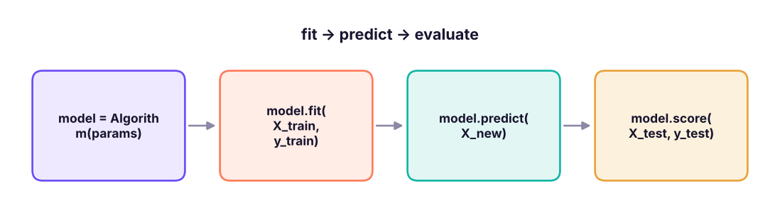
One consistent interface for every estimator.

Method	Available on	Does
`fit(X, y)`	Every estimator	Learns parameters from training data
`predict(X)`	Models	Predicted labels or values
`predict_proba(X)`	Most classifiers	Class probabilities
`transform(X)`	Transformers (scalers, encoders, PCA)	Converts features using fitted parameters
`fit_transform(X)`	Transformers	Fit then transform (training data only!)
`score(X, y)`	Models	Default metric (accuracy or R²)
`get_params()` / `set_params()`	All	Hyperparameters

X is a 2-D table of features (DataFrame or array, shape n_samples × n_features); y is a 1-D target.

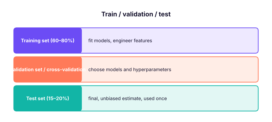
Train/test split

We judge a model on data it has never seen. Hold out a test set before doing anything else.

Python

import pandas as pd, numpy as np
from sklearn.model_selection import train_test_split
tc = pd.read_csv("telecom_churn.csv")
X = tc.drop(columns=["customer_id", "churn", "total_charges"])          # total_charges ≈ tenure × monthly: redundant
y = (tc["churn"] == "Yes").astype(int)
X_train, X_test, y_train, y_test = train_test_split(X, y, test_size=0.2, stratify=y, random_state=42)
print(X_train.shape, X_test.shape, f"churn rate train {y_train.mean():.3f} | test {y_test.mean():.3f}")

Output

(2400, 7) (600, 7) churn rate train 0.258 | test 0.257

Typical data splits. The test set is a final exam: use it once, at the end.

Option	Use
`test_size=0.2`	Hold out 20%
`stratify=y`	Keep the class balance the same in both sets (classification)
`random_state=42`	Reproducible split
Time-based split	For time series and anything predicted in the future: train on the past, test on the most recent period
Group split (`GroupShuffleSplit`)	Keep all rows of a customer/store in one set

Watch outNever tune on the test set

If you try many models and keep the one with the best test score, the test score is no longer an unbiased estimate. Choose with cross-validation on the training set (lesson 15); look at the test set once.

Baselines

A model is only useful if it beats a simple baseline.

Python

from sklearn.dummy import DummyClassifier, DummyRegressor
from sklearn.metrics import accuracy_score, recall_score
base = DummyClassifier(strategy="most_frequent").fit(X_train, y_train)
pred = base.predict(X_test)
print(f"always 'no churn': accuracy {accuracy_score(y_test, pred):.3f} | recall of churners {recall_score(y_test, pred):.3f}")
rule = ((X_test.contract == "Month-to-month") & (X_test.tenure_months <= 12)).astype(int)        # business rule from the EDA
print(f"rule 'new month-to-month': accuracy {accuracy_score(y_test, rule):.3f} | recall {recall_score(y_test, rule):.3f}")

Output

always 'no churn': accuracy 0.743 | recall of churners 0.000
rule 'new month-to-month': accuracy 0.777 | recall 0.240

74% accuracy by predicting "no churn" for everyone shows why accuracy alone is misleading for imbalanced problems (lesson 14).

Preprocessing with ColumnTransformer

Models need numbers on comparable scales. Numeric and categorical columns need different treatment.

Python

from sklearn.compose import ColumnTransformer
from sklearn.preprocessing import StandardScaler, OneHotEncoder
from sklearn.impute import SimpleImputer
from sklearn.pipeline import Pipeline, make_pipeline
num_cols = ["senior_citizen", "tenure_months", "monthly_charges", "support_calls"]
cat_cols = ["contract", "internet_service", "payment_method"]
prep = ColumnTransformer([
    ("num", make_pipeline(SimpleImputer(strategy="median"), StandardScaler()), num_cols),
    ("cat", make_pipeline(SimpleImputer(strategy="most_frequent"), OneHotEncoder(handle_unknown="ignore")), cat_cols),
])
Xt = prep.fit_transform(X_train)
print(Xt.shape, list(prep.get_feature_names_out())[:7], "...")

Output

(2400, 14) ['num__senior_citizen', 'num__tenure_months', 'num__monthly_charges', 'num__support_calls', 'cat__contract_Month-to-month', 'cat__contract_One year', 'cat__contract_Two year'] ...

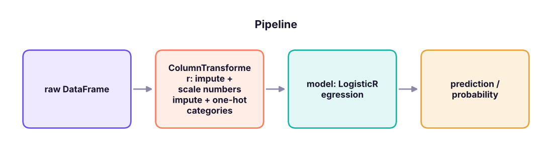
Pipelines: preprocessing + model as one object

Python

from sklearn.linear_model import LogisticRegression
from sklearn.ensemble import RandomForestClassifier, HistGradientBoostingClassifier
from sklearn.neighbors import KNeighborsClassifier
from sklearn.metrics import roc_auc_score
models = {"logistic regression": LogisticRegression(max_iter=1000), "k-nearest neighbours": KNeighborsClassifier(25),
          "random forest": RandomForestClassifier(300, min_samples_leaf=5, random_state=0), "gradient boosting": HistGradientBoostingClassifier(random_state=0)}
for name, model in models.items():
    pipe = Pipeline([("prep", prep), ("model", model)]).fit(X_train, y_train)
    proba = pipe.predict_proba(X_test)[:, 1]
    print(f"{name:22s} accuracy {pipe.score(X_test, y_test):.3f} | ROC-AUC {roc_auc_score(y_test, proba):.3f} | recall {recall_score(y_test, pipe.predict(X_test)):.3f}")

Output

logistic regression    accuracy 0.790 | ROC-AUC 0.803 | recall 0.396
k-nearest neighbours   accuracy 0.785 | ROC-AUC 0.759 | recall 0.344
random forest          accuracy 0.798 | ROC-AUC 0.793 | recall 0.403
gradient boosting      accuracy 0.760 | ROC-AUC 0.755 | recall 0.455

Why pipelines?

No leakage: scalers and imputers learn their statistics from the training data only, inside each fit (and inside every cross-validation fold).
One object to tune, save and deploy: raw data in, predictions out.
Less code and fewer mistakes when switching models.

A pipeline chains steps; fit runs fit_transform on each step, predict runs transform then predict.

A regression example

Python

from sklearn.linear_model import LinearRegression
from sklearn.metrics import mean_absolute_error, r2_score
h = pd.read_csv("house_prices.csv")
Xh, yh = h.drop(columns=["house_id", "price_lakh"]), h["price_lakh"]
Xh_tr, Xh_te, yh_tr, yh_te = train_test_split(Xh, yh, test_size=0.2, random_state=1)
prep_h = ColumnTransformer([("num", make_pipeline(SimpleImputer(strategy="median"), StandardScaler()), ["area_sqft", "bedrooms", "bathrooms", "age_years", "distance_to_center_km", "parking"]),
                            ("cat", OneHotEncoder(handle_unknown="ignore"), ["city"])])
for name, m in [("mean baseline", DummyRegressor()), ("linear regression", LinearRegression())]:
    p = Pipeline([("prep", prep_h), ("m", m)]).fit(Xh_tr, yh_tr).predict(Xh_te)
    print(f"{name:18s} MAE {mean_absolute_error(yh_te, p):6.2f} lakh | R² {r2_score(yh_te, p):.3f}")

Output

mean baseline      MAE  23.53 lakh | R² -0.005
linear regression  MAE   7.18 lakh | R² 0.900

Saving and loading a model

Python

import joblib, os
best = Pipeline([("prep", prep), ("model", LogisticRegression(max_iter=1000))]).fit(X_train, y_train)
joblib.dump(best, "churn_model.joblib")
loaded = joblib.load("churn_model.joblib")
new_customers = pd.DataFrame([{"senior_citizen": 0, "tenure_months": 3, "contract": "Month-to-month", "internet_service": "Fiber", "payment_method": "UPI", "monthly_charges": 95.0, "support_calls": 3},
                              {"senior_citizen": 1, "tenure_months": 60, "contract": "Two year", "internet_service": "DSL", "payment_method": "Auto-debit", "monthly_charges": 55.0, "support_calls": 0}])
print(loaded.predict_proba(new_customers)[:, 1].round(3), f"| file size {os.path.getsize('churn_model.joblib') / 1024:.0f} KB")
os.remove("churn_model.joblib")

Output

[0.864 0.008] | file size 5 KB

Save the whole pipeline, note the library versions (sklearn.__version__), and keep a model card (data, date, metrics, intended use). Load models only from sources you trust: joblib/pickle files can run code.

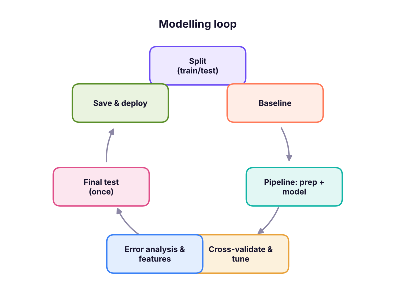
The workflow, end to end

The modelling loop you will repeat in every lesson of this track.

Summary

Key takeaways

Every estimator uses fit, then predict/predict_proba or transform; X is 2-D, y is 1-D.
Split first (stratified for classification, by time for forecasting); the test set is used once.
Always compare with a baseline (DummyClassifier, DummyRegressor, or a business rule).
ColumnTransformer + Pipeline apply the right preprocessing to each column type and prevent leakage.
Save the fitted pipeline with joblib and document versions and metrics.

Quick quiz6 questions · tap an answer to check it

1. Why use stratify=y in train_test_split?

Answer: A. Important for imbalanced classes.

2. Where should a StandardScaler learn its mean and standard deviation?

Answer: B. Fitting on all data leaks test information.

3. A churn model has 74% accuracy and churn is 26%. What can you say?

Answer: B. Compare with a baseline.

4. What does ColumnTransformer do?

Answer: A. e.g. scale numbers, one-hot encode categories.

5. Which split suits forecasting next month's demand?

Answer: B. Random splits leak the future into training.

6. What should you save for deployment?

Answer: B. One object turns raw data into predictions.

ExercisePractice

(1) Build a pipeline for hr_employees.csv that predicts attrition with logistic regression; compare it with a dummy baseline using ROC-AUC. (2) Add job_title as a categorical feature: does AUC change? (3) Save and reload the pipeline and score two made-up employees.

Show solution

Python

hr = pd.read_csv("hr_employees.csv")
y2 = (hr.attrition == "Yes").astype(int); X2 = hr.drop(columns=["emp_id", "attrition", "hire_date"])
nums = X2.select_dtypes("number").columns.tolist(); cats = [c for c in X2.columns if c not in nums]
p2 = Pipeline([("prep", ColumnTransformer([("n", StandardScaler(), nums), ("c", OneHotEncoder(handle_unknown="ignore"), cats)])), ("m", LogisticRegression(max_iter=2000))])
a, b, c, d = train_test_split(X2, y2, test_size=.2, stratify=y2, random_state=0)
print(roc_auc_score(d, p2.fit(a, c).predict_proba(b)[:, 1]), roc_auc_score(d, DummyClassifier().fit(a, c).predict_proba(b)[:, 1]))

Interview cornerQuestions you may be asked

Q: Why do we need a train/test split? To estimate how the model performs on new, unseen data; training performance is optimistic because the model has seen those examples.

Q: What is a pipeline and why use one? A chain of preprocessing steps and a model trained and applied as one object; it prevents leakage, simplifies tuning and makes deployment reliable.

Q: What is the difference between fit_transform and transform? fit_transform learns parameters (e.g. mean, categories) and applies them, used on training data; transform applies already-learned parameters, used on validation, test and new data.

Practise more online

Free, trusted places to test yourself on this topic. Links open the original site in a new tab.

← PreviousIntroduction to Machine Learning: Types, Business Framing and the ML Lifecycle Next →Data Preprocessing and Feature Engineering for ML