Statistics & Machine Learning · Lesson 12 of 28

Overfitting, Polynomial Regression and Regularisation (Ridge, Lasso, Elastic Net)

See overfitting and underfitting happen, learn the bias-variance trade-off with polynomial regression, and control model complexity with L2 (Ridge), L1 (Lasso) and Elastic Net penalties, including choosing the penalty strength with cross-validation, feature selection with Lasso, and learning curves.

● ML class 6✦ scikit-learn 1.7+Intermediate⏱ 110 min

⬇ Download PDF

By the end of this lesson you can

Recognise underfitting and overfitting from train vs test errors and plots
Explain the bias-variance trade-off and how model complexity affects it
Fit polynomial regression and control its degree
Apply Ridge, Lasso and Elastic Net and tune alpha with RidgeCV/LassoCV
Use learning and validation curves to decide between more data and a different model

Datasets used

house_prices.csv hr_employees.csv

Underfitting and overfitting

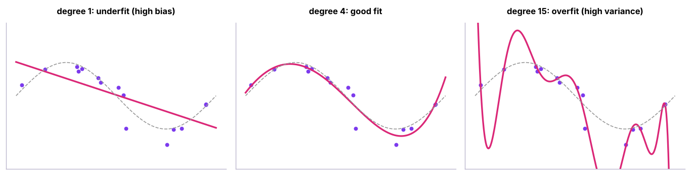
Polynomial models of degree 1, 4 and 15 on the same noisy data. Degree 1 underfits, degree 4 fits well, degree 15 chases noise.

	Underfitting	Good fit	Overfitting
Training error	High	Low	Very low
Test error	High	Low	High
Cause	Model too simple, missing features		Model too complex, too little data, leakage
Fix	More features, more flexible model, less regularisation		More data, simpler model, regularisation, feature selection, early stopping

The bias-variance trade-off

Bias is the error from wrong assumptions (a line for a curve). Variance is the error from sensitivity to the particular training sample. Total expected error = bias² + variance + irreducible noise.

Python

from sklearn.metrics import mean_squared_error
x_test = rng.uniform(0, 1, 500); y_test = np.sin(2 * np.pi * x_test) + rng.normal(0, .25, 500)
for d in (1, 2, 3, 4, 6, 9, 12, 15):
    m = make_pipeline(PolynomialFeatures(d), StandardScaler(), LinearRegression()).fit(x[:, None], y)
    tr = mean_squared_error(y, m.predict(x[:, None])); te = mean_squared_error(y_test, m.predict(x_test[:, None]))
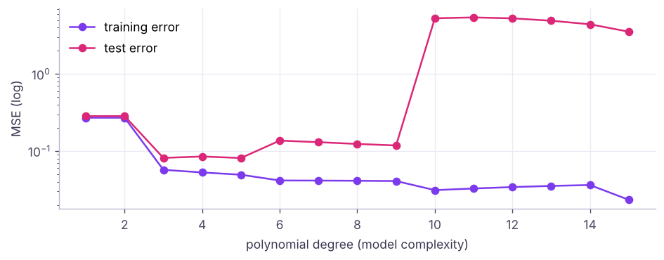
    print(f"degree {d:2d}: train MSE {tr:7.3f} | test MSE {te:10.3f}")

Output

degree  1: train MSE   0.271 | test MSE      0.284
degree  2: train MSE   0.271 | test MSE      0.285
degree  3: train MSE   0.057 | test MSE      0.082
degree  4: train MSE   0.053 | test MSE      0.085
degree  6: train MSE   0.042 | test MSE      0.137
degree  9: train MSE   0.041 | test MSE      0.118
degree 12: train MSE   0.034 | test MSE      5.285
degree 15: train MSE   0.023 | test MSE      3.548

As complexity grows, training error keeps falling while test error falls then rises: the sweet spot is in between.

Regularisation

Instead of choosing fewer features by hand, add a penalty on large coefficients to the cost:

\text{Ridge (L2):}\; J = \text{MSE} + \alpha\sum_j w_j^2 \qquad \text{Lasso (L1):}\; J = \text{MSE} + \alpha\sum_j |w_j|

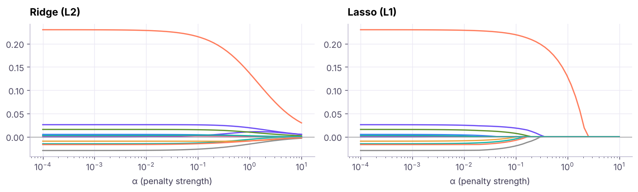
Elastic Net mixes both (l1_ratio). Larger α means stronger shrinkage, simpler models, more bias and less variance. Always scale features first, so the penalty treats them fairly.

Python

for name, model in [("no penalty", LinearRegression()), ("Ridge α=0.01", Ridge(alpha=0.01)), ("Lasso α=0.001", Lasso(alpha=0.001, max_iter=100000))]:
    m = make_pipeline(PolynomialFeatures(15), StandardScaler(), model).fit(x[:, None], y)
    coefs = m[-1].coef_
    print(f"degree-15 {name:12s} test MSE {mean_squared_error(y_test, m.predict(x_test[:, None])):9.3f} | largest |coef| {np.abs(coefs).max():12.1f} | zero coefs {(np.abs(coefs) < 1e-8).sum():2d} of {len(coefs)}")

Output

degree-15 no penalty   test MSE     3.548 | largest |coef|       9560.9 | zero coefs  0 of 16
degree-15 Ridge α=0.01 test MSE     0.113 | largest |coef|          2.2 | zero coefs  1 of 16
degree-15 Lasso α=0.001 test MSE     0.089 | largest |coef|          4.1 | zero coefs 12 of 16

The same degree-15 model becomes well behaved once its coefficients are penalised. Lasso sets some coefficients exactly to zero (automatic feature selection); Ridge shrinks all of them smoothly and handles correlated features well.

Coefficient paths: as α grows, Ridge shrinks every coefficient gradually while Lasso drops features to exactly zero one by one.

Choosing α with cross-validation

Python

from sklearn.model_selection import train_test_split, cross_val_score
h = pd.read_csv("house_prices.csv").dropna(subset=["area_sqft"])
pps = h.price_lakh * 1e5 / h.area_sqft; h = h[pps.between(pps.median() / 3, pps.median() * 3)]
X = pd.get_dummies(h.drop(columns=["house_id", "price_lakh"]), columns=["city"], drop_first=True).astype(float); yv = h.price_lakh
Xtr, Xte, ytr, yte = train_test_split(X, yv, test_size=0.2, random_state=0)
poly = lambda est: make_pipeline(PolynomialFeatures(2, include_bias=False), StandardScaler(), est)
models = {"linear (degree 2)": poly(LinearRegression()), "RidgeCV": poly(RidgeCV(alphas=np.logspace(-3, 3, 30))),
          "LassoCV": poly(LassoCV(cv=5, random_state=0, max_iter=50000)), "ElasticNet": poly(ElasticNet(alpha=0.05, l1_ratio=0.5, max_iter=50000))}
for name, m in models.items():
    m.fit(Xtr, ytr); cv = cross_val_score(m, Xtr, ytr, cv=5, scoring="neg_root_mean_squared_error").mean()
    extra = f" | α = {m[-1].alpha_:.4g}" if hasattr(m[-1], "alpha_") else ""
    nz = f" | non-zero coefs {(m[-1].coef_ != 0).sum()} of {len(m[-1].coef_)}"
    print(f"{name:18s} CV RMSE {-cv:6.2f} | test RMSE {mean_squared_error(yte, m.predict(Xte)) ** .5:6.2f}{extra}{nz}")

Output

linear (degree 2)  CV RMSE   7.21 | test RMSE   7.72 | non-zero coefs 51 of 54
RidgeCV            CV RMSE   7.20 | test RMSE   7.75 | α = 0.788 | non-zero coefs 53 of 54
LassoCV            CV RMSE   7.08 | test RMSE   7.64 | α = 0.07792 | non-zero coefs 25 of 54
ElasticNet         CV RMSE   7.41 | test RMSE   8.05 | non-zero coefs 45 of 54

With about 900 training rows and 54 polynomial features, all models perform similarly here; Lasso reaches the same accuracy with far fewer terms. Regularisation matters most when features are many relative to rows, or strongly correlated.

Learning curves: more data or a better model?

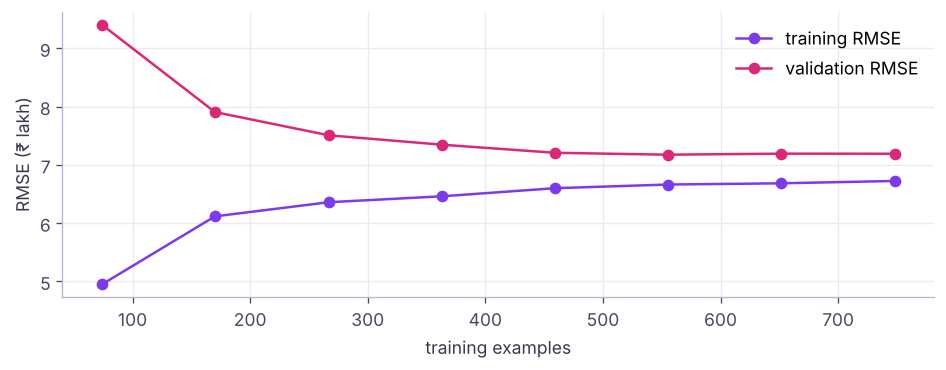
Learning curves for a degree-2 Ridge model on house prices: the training and validation errors converge as data grows, so more data would help little; a more flexible model or better features would help more.

Learning-curve pattern	Diagnosis	Action
Both errors high and close	High bias (underfitting)	More features, more complex model
Big gap: low train, high validation	High variance (overfitting)	More data, regularisation, simpler model
Gap closing as data grows	Variance falling	Collect more data

Regularisation beyond linear models

Model	Regularisation knobs
Logistic regression	`C` = 1/α (smaller C = stronger penalty), `penalty="l1"/"l2"/"elasticnet"`
Decision trees	`max_depth`, `min_samples_leaf`, pruning (`ccp_alpha`)
Random forests / boosting	Tree depth, number of trees, learning rate, subsampling
Neural networks	Weight decay (L2), dropout, early stopping, data augmentation
KNN	Larger k = smoother

Summary

Key takeaways

Underfitting: high error everywhere (bias). Overfitting: low training error, high test error (variance).
Polynomial features add flexibility; the degree controls the bias-variance trade-off.
Ridge (L2) shrinks coefficients; Lasso (L1) zeroes some (feature selection); Elastic Net combines them. Scale features first.
Pick α by cross-validation (RidgeCV, LassoCV, GridSearchCV).
Learning curves tell you whether more data or a different model will help.

Quick quiz6 questions · tap an answer to check it

1. Training error 2%, test error 25%. Diagnosis?

Answer: B. The model memorised the training data.

2. Which penalty can set coefficients exactly to zero?

Answer: B. L1 performs feature selection.

3. What happens as α increases in Ridge regression?

Answer: A. Stronger penalty = simpler model.

4. Why scale features before regularisation?

Answer: A. Otherwise large-unit features are under-penalised.

5. In logistic regression in scikit-learn, a smaller C means…

Answer: A. C is the inverse of α.

6. Learning curves show training and validation errors both high and close together. What helps?

Answer: B. This is high bias.

ExercisePractice

(1) Plot validation curves (validation_curve) of Ridge alpha for the house data. (2) Fit LogisticRegressionCV with L1 penalty on the HR attrition data: which features survive? (3) Compare degree 1, 2 and 3 polynomial Ridge models with 5-fold CV.

Show solution

Python

from sklearn.model_selection import validation_curve
from sklearn.linear_model import LogisticRegressionCV
al = np.logspace(-3, 3, 13)
tr_, va_ = validation_curve(poly(Ridge()), Xtr, ytr, param_name="ridge__alpha", param_range=al, cv=5, scoring="neg_root_mean_squared_error")
yb = (hr.attrition == "Yes").astype(int)
lr1 = LogisticRegressionCV(penalty="l1", solver="saga", Cs=10, cv=5, max_iter=5000).fit(StandardScaler().fit_transform(Xh), yb)
print(Xh.columns[lr1.coef_[0] != 0].tolist())
for d in (1, 2, 3): print(d, cross_val_score(make_pipeline(PolynomialFeatures(d, include_bias=False), StandardScaler(), Ridge(1)), Xtr, ytr, cv=5, scoring="r2").mean())

Interview cornerQuestions you may be asked

Q: Explain the bias-variance trade-off. Simple models have high bias (systematic error) and low variance; complex models have low bias but high variance (sensitivity to the training sample). We choose complexity that minimises total error on new data.

Q: L1 vs L2 regularisation? L2 shrinks coefficients towards zero and handles correlated features; L1 can set coefficients exactly to zero, selecting features; Elastic Net combines both.

Q: How do you detect overfitting? Compare training and validation/test performance (large gap), use cross-validation, and inspect learning curves.

Practise more online

Free, trusted places to test yourself on this topic. Links open the original site in a new tab.

← PreviousGradient Descent: How Models Learn (Built from Scratch in NumPy)Next →Logistic Regression: Probabilities, Odds Ratios and Credit-Risk Scoring