
K-Nearest Neighbours: Classifier and Regressor (Bank Loans Case Study)
The simplest learning algorithm: predict from the most similar past examples. Distance metrics, choosing k, why scaling is essential, weighted voting, the curse of dimensionality, KNN for classification and regression, tuning with GridSearchCV, and the full Bank Loans case study from the live class with metrics and scoring of new applicants.
- Explain how KNN classifies and regresses using distances to neighbours
- Compute Euclidean, Manhattan and Minkowski distances and know why scaling matters
- Choose k and weighting with cross-validation and explain the bias-variance effect of k
- Run the Bank Loans case study end to end with a pipeline and GridSearchCV
- Describe KNN's strengths, weaknesses and the curse of dimensionality
The idea
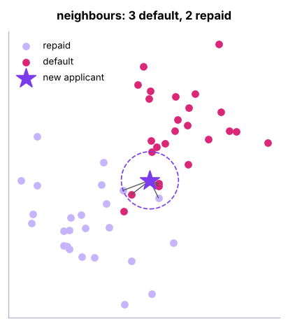
"Tell me who your neighbours are, and I'll tell you who you are." To predict a new point, find the k most similar labelled points and let them vote (classification) or average their values (regression). There is no training beyond storing the data, so KNN is a lazy, instance-based learner.
Distances

Minkowski distance generalises both (p=2 Euclidean, p=1 Manhattan). Cosine distance suits text and embeddings; Hamming suits binary features.
from scipy.spatial import distance
x1, x2 = np.array([30, 45.0, 8.5]), np.array([42, 60.0, 12.0])          # age, income (thousands), debt-to-income %
print("Euclidean", round(distance.euclidean(x1, x2), 2), "| Manhattan", distance.cityblock(x1, x2), "| cosine", round(distance.cosine(x1, x2), 4))Euclidean 19.53 | Manhattan 30.5 | cosine 0.0003
Why scaling is essential
b = pd.read_csv("bank_loans.csv")
known = b[b.default.notna()].copy(); known["default"] = known.default.astype(int); new_apps = b[b.default.isna()].copy()
feats = ["age", "ed", "employ", "address", "income", "debtinc", "creddebt", "othdebt"]
print(known[feats].describe().loc[["mean", "std", "max"]].round(1))age ed employ address income debtinc creddebt othdebt mean 37.4 1.9 6.3 5.3 49.5 10.0 1.7 3.3 std 10.6 1.0 5.9 5.0 24.9 6.5 1.7 3.4 max 55.0 5.0 24.0 22.0 172.4 41.0 12.3 43.0
Income ranges up to 170 while ed ranges 1–5: unscaled, income dominates every distance and education is ignored. Standardise (or min-max scale) before KNN.
Choosing k
| Small k | Large k |
|---|---|
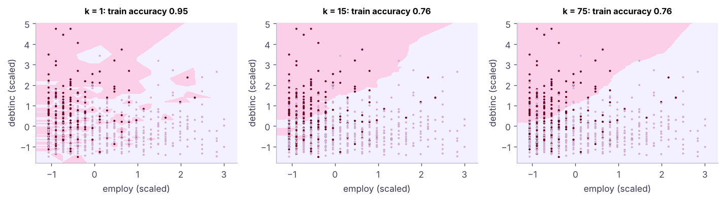
| Flexible, low bias, high variance (overfits) | Smooth, high bias, low variance (underfits) |
| k = 1 memorises training data (100% train accuracy) | k = n predicts the majority class everywhere |
Rules of thumb: start near √n, prefer odd k for binary problems (no ties), and choose by cross-validation. weights="distance" lets closer neighbours count more.
Case study: Bank Loans
Business problem: decide which of 150 new loan applicants to approve, using 700 past customers with known outcomes.
from sklearn.model_selection import train_test_split, GridSearchCV, StratifiedKFold
from sklearn.metrics import roc_auc_score, classification_report, confusion_matrix, accuracy_score
X, y = known[feats], known.default
Xtr, Xte, ytr, yte = train_test_split(X, y, test_size=0.3, stratify=y, random_state=42)
raw = KNeighborsClassifier(15).fit(Xtr, ytr); scaled = make_pipeline(StandardScaler(), KNeighborsClassifier(15)).fit(Xtr, ytr)
print(f"k=15 without scaling: AUC {roc_auc_score(yte, raw.predict_proba(Xte)[:, 1]):.3f} | with scaling: AUC {roc_auc_score(yte, scaled.predict_proba(Xte)[:, 1]):.3f}")k=15 without scaling: AUC 0.757 | with scaling: AUC 0.765
Scaling helps only a little here, because the large-range features (income, debt-to-income) happen to be informative anyway. When a large-range feature is irrelevant (for example a customer ID number or a postcode), unscaled KNN can fail completely.
pipe = make_pipeline(StandardScaler(), KNeighborsClassifier())
grid = {"kneighborsclassifier__n_neighbors": list(range(3, 62, 4)), "kneighborsclassifier__weights": ["uniform", "distance"], "kneighborsclassifier__metric": ["euclidean", "manhattan"]}
gs = GridSearchCV(pipe, grid, cv=StratifiedKFold(5, shuffle=True, random_state=0), scoring="roc_auc", n_jobs=-1).fit(Xtr, ytr)
print("best:", {k.split("__")[1]: v for k, v in gs.best_params_.items()}, f"| CV AUC {gs.best_score_:.3f}")
p = gs.predict_proba(Xte)[:, 1]
print(f"test AUC {roc_auc_score(yte, p):.3f} | accuracy at 0.5 {accuracy_score(yte, p >= .5):.3f}")
print(confusion_matrix(yte, p >= 0.5))
print(classification_report(yte, p >= 0.5, target_names=["repaid", "default"], digits=3))best: {'metric': 'manhattan', 'n_neighbors': 51, 'weights': 'distance'} | CV AUC 0.772
test AUC 0.810 | accuracy at 0.5 0.733
[[134 9]
[ 47 20]]
precision recall f1-score support
repaid 0.740 0.937 0.827 143
default 0.690 0.299 0.417 67
accuracy 0.733 210
macro avg 0.715 0.618 0.622 210
weighted avg 0.724 0.733 0.696 210t = 0.3 # lower threshold: missing a defaulter is costlier
print(f"threshold {t}:"); print(confusion_matrix(yte, p >= t)); print(classification_report(yte, p >= t, target_names=["repaid", "default"], digits=3))threshold 0.3:
[[94 49]
[ 9 58]]
precision recall f1-score support
repaid 0.913 0.657 0.764 143
default 0.542 0.866 0.667 67
accuracy 0.724 210
macro avg 0.727 0.762 0.715 210
weighted avg 0.794 0.724 0.733 210KNN vs logistic regression
from sklearn.linear_model import LogisticRegression
from sklearn.model_selection import cross_val_score
cv = StratifiedKFold(5, shuffle=True, random_state=0)
for name, m in [("KNN (tuned)", gs.best_estimator_), ("logistic regression", make_pipeline(StandardScaler(), LogisticRegression(max_iter=1000)))]:
s = cross_val_score(m, X, y, cv=cv, scoring="roc_auc"); print(f"{name:20s} 5-fold AUC {s.mean():.3f} ± {s.std():.3f}")KNN (tuned) 5-fold AUC 0.786 ± 0.046 logistic regression 5-fold AUC 0.803 ± 0.042
On this small, roughly linear credit problem, logistic regression is as good or better, and far easier to explain. KNN shines when the boundary is irregular and the data are dense.
Scoring new applicants and explaining with neighbours
best = gs.best_estimator_.fit(X, y)
new_apps["p_default"] = best.predict_proba(new_apps[feats])[:, 1].round(3)
print(new_apps.p_default.describe().round(3).to_dict())
app = new_apps.sort_values("p_default", ascending=False).iloc[0]
dist_, idx = best[-1].kneighbors(best[0].transform(app[feats].to_frame().T.astype(float)), n_neighbors=5)
print(f"{app.customer_id}: P(default) {app.p_default:.2f}. Its 5 most similar past customers:")
print(known.iloc[idx[0]][feats + ["default"]].to_string(index=False)){'count': 150.0, 'mean': 0.295, 'std': 0.176, 'min': 0.016, '25%': 0.168, '50%': 0.271, '75%': 0.401, 'max': 0.802}
L0782: P(default) 0.80. Its 5 most similar past customers:
age ed employ address income debtinc creddebt othdebt default
35 2 1 5 33.7 30.7 3.24 7.11 1
47 2 0 4 26.5 32.8 4.28 4.41 1
40 1 3 4 49.7 24.1 4.34 7.64 1
39 1 5 4 32.7 24.3 3.44 4.51 1
26 1 1 2 52.2 29.4 5.63 9.72 1KNN explanations are concrete: here, all five of the most similar past customers defaulted.
KNN regression
from sklearn.neighbors import KNeighborsRegressor
from sklearn.metrics import mean_absolute_error
h = pd.read_csv("house_prices.csv").dropna(subset=["area_sqft"])
hf = ["area_sqft", "bedrooms", "bathrooms", "age_years", "distance_to_center_km"]
Htr, Hte, htr, hte = train_test_split(h[hf], h.price_lakh, test_size=0.2, random_state=0)
for k in (1, 5, 15, 40):
    m = make_pipeline(StandardScaler(), KNeighborsRegressor(k, weights="distance")).fit(Htr, htr)
print(f"k = {k:2d}: test MAE {mean_absolute_error(hte, m.predict(Hte)):.2f} lakh")k = 1: test MAE 16.40 lakh k = 5: test MAE 12.57 lakh k = 15: test MAE 12.96 lakh k = 40: test MAE 12.42 lakh
Strengths, weaknesses and the curse of dimensionality
| Strengths | Weaknesses |
|---|---|
| Simple, intuitive, no training | Slow predictions on large data (must search all points) |
| Naturally multiclass; non-linear boundaries | Needs scaling; sensitive to irrelevant features |
| Explanations by example | Struggles in high dimensions |
| Works for regression too | Memory: stores the whole training set |
rng = np.random.default_rng(0)
for dims in (2, 10, 100, 1000):
    pts_ = rng.uniform(size=(500, dims)); d = np.linalg.norm(pts_[1:] - pts_[0], axis=1)
print(f"{dims:4d} dimensions: nearest/farthest distance ratio {d.min() / d.max():.2f}")2 dimensions: nearest/farthest distance ratio 0.01 10 dimensions: nearest/farthest distance ratio 0.30 100 dimensions: nearest/farthest distance ratio 0.73 1000 dimensions: nearest/farthest distance ratio 0.90
In high dimensions every point is almost equally far from every other (the ratio approaches 1), so "nearest" stops meaning "similar". Reduce dimensions (feature selection, PCA) first. For millions of vectors (embeddings in RAG systems, GenAI track), approximate nearest-neighbour indexes (FAISS, HNSW) make search fast.
Summary
- KNN predicts from the k most similar labelled examples: majority vote or (weighted) average.
- Distances: Euclidean, Manhattan, Minkowski, cosine; always scale features first.
- Small k overfits, large k underfits; tune k, weights and metric with cross-validation.
- Bank Loans: a scaled, tuned KNN reaches a decent AUC, and logistic regression is as good and more interpretable on this data.
- KNN suffers from slow prediction and the curse of dimensionality; approximate nearest-neighbour search powers vector databases.
1. What does KNN do during training?
2. Why must features be scaled for KNN?
3. What happens with k = 1?
4. Which distance is Minkowski with p = 1?
5. What is the curse of dimensionality for KNN?
6. How does weights="distance" change predictions?
(1) Use KNN to predict churn on telecom_churn.csv (one-hot + scale) and tune k with GridSearchCV; compare AUC with logistic regression. (2) Plot test MAE against k (1–50) for KNN regression on house prices. (3) Find the 5 nearest neighbours of a new house (1,400 sq ft, 3 bed, 2 bath, 8 years, 6 km).
Show solution
from sklearn.compose import ColumnTransformer
from sklearn.preprocessing import OneHotEncoder
tc = pd.read_csv("telecom_churn.csv"); Xc = tc.drop(columns=["customer_id", "churn", "total_charges"]); yc = (tc.churn == "Yes").astype(int)
pre = ColumnTransformer([("n", StandardScaler(), ["senior_citizen", "tenure_months", "monthly_charges", "support_calls"]), ("c", OneHotEncoder(), ["contract", "internet_service", "payment_method"])])
g = GridSearchCV(make_pipeline(pre, KNeighborsClassifier()), {"kneighborsclassifier__n_neighbors": range(5, 120, 10)}, cv=5, scoring="roc_auc").fit(Xc, yc); print(g.best_params_, g.best_score_)
maes = [mean_absolute_error(hte, make_pipeline(StandardScaler(), KNeighborsRegressor(k)).fit(Htr, htr).predict(Hte)) for k in range(1, 51)]
m = make_pipeline(StandardScaler(), KNeighborsRegressor(5)).fit(h[hf], h.price_lakh)
print(m.predict(pd.DataFrame([[1400, 3, 2, 8, 6]], columns=hf)))Q: How does KNN work and how do you choose k? It finds the k closest training points by a distance metric and votes or averages; choose k (and weighting, metric) by cross-validation, balancing overfitting (small k) and oversmoothing (large k).
Q: What are the disadvantages of KNN? Slow and memory-heavy predictions, sensitivity to scaling and irrelevant features, poor performance in high dimensions, and imbalanced classes skew votes.
Q: How would you speed up nearest-neighbour search on millions of points? KD-trees or ball trees for low dimensions, and approximate nearest-neighbour indexes (HNSW, FAISS, ScaNN) for high-dimensional embeddings.
Practise more online
Free, trusted places to test yourself on this topic. Links open the original site in a new tab.