
Hypothesis Testing I: The Framework, p-values, z-tests and t-tests
Turn business questions into testable hypotheses. Null and alternative hypotheses, significance level, test statistics, p-values and critical values, one- vs two-tailed tests, Type I and II errors and power, then one-sample, two-sample (Welch) and paired t-tests and z-tests for proportions, on a delivery-time case study.
- Translate a business question into null and alternative hypotheses
- Explain significance level, test statistic, p-value and critical value, and decide with both
- Choose one- or two-tailed tests and describe Type I/II errors and power
- Run and interpret one-sample, independent (Welch) and paired t-tests and a z-test for proportions
- Report effect sizes and confidence intervals, not just p-values
From business question to hypothesis
Case. A quick-commerce company promises "delivery in 30 minutes". Operations claim Pune meets the promise on average. Is the average delivery time in Pune really 30 minutes, or is it slower? Is Hyderabad different from Pune?
A hypothesis test checks whether data are consistent with a default claim.
| Term | Meaning | Delivery case |
|---|---|---|
| H₀ (null) | No effect / status quo; assumed true until evidence | μ_Pune = 30 min |
| H₁ (alternative) | What we want evidence for | μ_Pune > 30 min (one-tailed) or ≠ 30 (two-tailed) |
| α (significance level) | Accepted risk of a false alarm | 0.05 |
| Test statistic | Distance from H₀ in standard-error units | t = (x̄ − 30)/(s/√n) |
| p-value | P(data at least this extreme | H₀ true) | from the t distribution |
| Decision | p ≤ α → reject H₀; p > α → fail to reject H₀ |

p-values and critical values
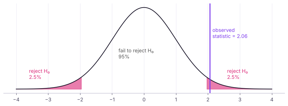
print("critical values: two-tailed z ±", round(stats.norm.ppf(0.975), 3), "| one-tailed z", round(stats.norm.ppf(0.95), 3), "| two-tailed t(df=59) ±", round(stats.t.ppf(0.975, 59), 3))
for z in (1.2, 1.7, 2.06, 3.1): print(f"z = {z}: two-tailed p = {2 * stats.norm.sf(abs(z)):.4f} | one-tailed p = {stats.norm.sf(z):.4f}")critical values: two-tailed z ± 1.96 | one-tailed z 1.645 | two-tailed t(df=59) ± 2.001 z = 1.2: two-tailed p = 0.2301 | one-tailed p = 0.1151 z = 1.7: two-tailed p = 0.0891 | one-tailed p = 0.0446 z = 2.06: two-tailed p = 0.0394 | one-tailed p = 0.0197 z = 3.1: two-tailed p = 0.0019 | one-tailed p = 0.0010
It is not the probability that H₀ is true, and 1 − p is not the probability that H₁ is true. A large p-value does not prove H₀ ("absence of evidence is not evidence of absence"). A tiny p-value does not mean a large or important effect.
One- vs two-tailed
| Two-tailed | One-tailed | |
|---|---|---|
| H₁ | μ ≠ 30 (any difference) | μ > 30 (only "slower") |
| α split | 2.5% in each tail | 5% in one tail |
| When | Default; direction unknown | Direction fixed before looking at data, and the other direction is irrelevant |
Errors and power
| H₀ true | H₀ false | |
|---|---|---|
| Reject H₀ | Type I error (false positive), probability α | Correct: power = 1 − β |
| Fail to reject | Correct | Type II error (false negative), probability β |
Fire alarm analogy: a Type I error rings without a fire; a Type II error stays silent during a fire. Lower α means fewer false alarms but more misses unless you collect more data. Power (commonly 80%) grows with sample size, effect size and α.
One-sample t-test: does Pune meet 30 minutes?
import pandas as pd
d = pd.read_csv("delivery_times.csv")
pune, hyd = d[d.city == "Pune"].delivery_minutes, d[d.city == "Hyderabad"].delivery_minutes
print(f"Pune: n={len(pune)}, mean {pune.mean():.2f}, sd {pune.std():.2f}")
t_two = stats.ttest_1samp(pune, 30)
t_one = stats.ttest_1samp(pune, 30, alternative="greater")
se = pune.std() / np.sqrt(len(pune))
print(f"t = {t_two.statistic:.3f}, df = {len(pune) - 1} | two-tailed p = {t_two.pvalue:.4f} | one-tailed (greater) p = {t_one.pvalue:.4f}")
print(f"by hand: t = ({pune.mean():.2f} − 30) / {se:.3f} = {(pune.mean() - 30) / se:.3f}")
ci = stats.t.interval(0.95, len(pune) - 1, loc=pune.mean(), scale=se)
print(f"95% CI for mean: {ci[0]:.2f} to {ci[1]:.2f} minutes (30 is {'outside' if not ci[0] <= 30 <= ci[1] else 'inside'})")
print(f"effect size (Cohen's d) = {(pune.mean() - 30) / pune.std():.2f}")Pune: n=60, mean 31.70, sd 6.39 t = 2.060, df = 59 | two-tailed p = 0.0439 | one-tailed (greater) p = 0.0219 by hand: t = (31.70 − 30) / 0.825 = 2.060 95% CI for mean: 30.05 to 33.35 minutes (30 is outside) effect size (Cohen's d) = 0.27
Conclusion. At α = 0.05 we reject H₀: Pune's average delivery time (about 31.7 minutes) is statistically higher than the 30-minute promise (p ≈ 0.02 one-tailed). The difference is small (under 2 minutes, d ≈ 0.27), so the business question is whether 1–2 minutes matter to customers, not just whether p < 0.05.
Two-sample t-test: Pune vs Hyderabad
print(f"Hyderabad: n={len(hyd)}, mean {hyd.mean():.2f}, sd {hyd.std():.2f}")
lev = stats.levene(pune, hyd); print(f"Levene test for equal variances p = {lev.pvalue:.3f} → {'unequal' if lev.pvalue < 0.05 else 'equal'} variances")
w = stats.ttest_ind(hyd, pune, equal_var=False)             # Welch's t-test: safe default
print(f"Welch t = {w.statistic:.3f}, p = {w.pvalue:.4f}, difference = {hyd.mean() - pune.mean():.2f} min")
pooled = np.sqrt(((len(pune) - 1) * pune.var() + (len(hyd) - 1) * hyd.var()) / (len(pune) + len(hyd) - 2))
print(f"Cohen's d = {(hyd.mean() - pune.mean()) / pooled:.2f}")Hyderabad: n=55, mean 33.81, sd 7.60 Levene test for equal variances p = 0.047 → unequal variances Welch t = 1.601, p = 0.1123, difference = 2.11 min Cohen's d = 0.30
Conclusion. p ≈ 0.11 > 0.05: we fail to reject H₀. The data do not show a significant difference between the cities (Hyderabad is about 2 minutes slower in this sample, but that could be chance). Use Welch's test (equal_var=False) by default: it does not assume equal variances and loses almost nothing when they are equal.
Paired t-test: before and after
Use a paired test when the same units are measured twice (same riders before/after training, same stores before/after a layout change).
rng = np.random.default_rng(5)
before = rng.normal(34, 5, 30).round(1)
after = (before - rng.normal(1.5, 1.5, 30)).round(1)          # simulated route-training effect
pt = stats.ttest_rel(before, after)
it = stats.ttest_ind(before, after, equal_var=False)
print(f"mean improvement {np.mean(before - after):.2f} min | paired p = {pt.pvalue:.4f} | (wrong) independent p = {it.pvalue:.4f}")mean improvement 1.17 min | paired p = 0.0003 | (wrong) independent p = 0.3342
Pairing removes rider-to-rider variation, so the same improvement is detected far more clearly.
z-test for proportions
from statsmodels.stats.proportion import proportions_ztest
hr = pd.read_csv("hr_employees.csv")
ot = hr[hr.overtime == "Yes"].attrition.eq("Yes"); no = hr[hr.overtime == "No"].attrition.eq("Yes")
stat, p = proportions_ztest([ot.sum(), no.sum()], [len(ot), len(no)])
print(f"attrition: overtime {ot.mean():.1%} (n={len(ot)}) vs no overtime {no.mean():.1%} (n={len(no)}) | z = {stat:.2f}, p = {p:.2e}")
stat1, p1 = proportions_ztest(hr.attrition.eq("Yes").sum(), len(hr), value=0.20, alternative="larger")
print(f"is company attrition above the 20% industry benchmark? z = {stat1:.2f}, p = {p1:.2e}")attrition: overtime 36.7% (n=433) vs no overtime 21.6% (n=1067) | z = 6.07, p = 1.26e-09 is company attrition above the 20% industry benchmark? z = 5.24, p = 7.89e-08
Choosing a test (means)
| Situation | Test | Python |
|---|---|---|
| One mean vs a target, σ unknown | One-sample t | stats.ttest_1samp |
| Two independent groups | Welch's t | stats.ttest_ind(..., equal_var=False) |
| Same units twice | Paired t | stats.ttest_rel |
| One or two proportions | z-test | statsmodels proportions_ztest |
| Non-normal small samples | Mann-Whitney U / Wilcoxon (next lesson) | stats.mannwhitneyu, stats.wilcoxon |
| 3+ groups | ANOVA (next lesson) | stats.f_oneway |
Assumptions for t-tests: independent observations, roughly normal data or large samples (CLT), and for the pooled version equal variances.
Reporting
Pune deliveries averaged 31.7 minutes (95% CI 30.1–33.4, n = 60), significantly above the 30-minute promise (one-sample t = 2.06, one-tailed p = 0.022). The gap is small (d = 0.27). Recommendation: monitor the share of orders above 40 minutes (13%) rather than the average.
Report the estimate, CI, test, p-value, effect size and business meaning.
Summary
- H₀ is the default (no effect); H₁ is what you want evidence for; fix α (usually 0.05) and the tails before looking.
- p-value = probability of data this extreme if H₀ were true; reject H₀ when p ≤ α (equivalently when the statistic passes the critical value).
- Type I (false positive, α) vs Type II (false negative, β); power = 1 − β grows with n and effect size.
- One-sample, Welch two-sample and paired t-tests compare means; z-tests compare proportions.
- Always report effect size and a confidence interval: statistical significance is not business significance.
1. The p-value is 0.03 and α = 0.05. What do you conclude?
2. Which is a Type I error?
3. Which test compares the same riders before and after training?
4. Why prefer Welch's t-test for two groups?
equal_var=False.5. p = 0.40. What can you say?
6. What increases the power of a test?
(1) Test whether Hyderabad's mean delivery time exceeds 30 minutes. (2) Test whether employees who left had lower monthly income than those who stayed (one-tailed Welch). Report the difference and d. (3) Test whether the share of overtime workers differs between Sales and IT.
Show solution
print(stats.ttest_1samp(hyd, 30, alternative="greater"))
left, stay = hr[hr.attrition == "Yes"].monthly_income, hr[hr.attrition == "No"].monthly_income
r = stats.ttest_ind(left, stay, equal_var=False, alternative="less"); print(r, left.mean() - stay.mean())
print((left.mean() - stay.mean()) / np.sqrt((left.var() + stay.var()) / 2))
s_, i_ = hr[hr.department == "Sales"].overtime.eq("Yes"), hr[hr.department == "IT"].overtime.eq("Yes")
print(proportions_ztest([s_.sum(), i_.sum()], [len(s_), len(i_)]))Q: Explain a p-value to a business stakeholder. If there were truly no difference, how surprising would our data be? A p-value of 0.01 means a result this extreme would happen only 1% of the time by chance alone.
Q: What is the difference between statistical and practical significance? Statistical significance says an effect is unlikely to be zero; practical significance asks whether it is large enough to matter (effect size, cost, revenue).
Q: How do you choose α? By the cost of errors: 0.05 by convention; lower (0.01) when false positives are expensive (medical, financial launches); sometimes higher for early exploration.
Practise more online
Free, trusted places to test yourself on this topic. Links open the original site in a new tab.