Statistics & Machine Learning · Lesson 18 of 28

Ensembles I: Bagging and Random Forests

Combine many models to beat one. The wisdom of crowds, bootstrap aggregating (bagging), random forests with feature subsampling, out-of-bag evaluation, the key hyperparameters, feature importance (impurity vs permutation), extra trees, voting and stacking ensembles, applied to telecom churn.

● ML track (added)✦ scikit-learn 1.7+Intermediate⏱ 100 min

⬇ Download PDF

By the end of this lesson you can

Explain why averaging many diverse models reduces variance
Build bagging and random-forest models and use out-of-bag scores
Tune n_estimators, max_features, max_depth and min_samples_leaf
Compare impurity-based and permutation feature importance
Combine different models with voting and stacking

Datasets used

telecom_churn.csv house_prices.csv

Why ensembles work

If each of many independent models is right 65% of the time, a majority vote of them is right far more often. Errors cancel when models make different mistakes.

Python

import numpy as np, pandas as pd
from scipy.stats import binom
for n in (1, 5, 25, 101):
    print(f"{n:3d} independent voters, each 65% accurate → majority correct {binom.sf(n // 2, n, 0.65):.3f}")

Output

  1 independent voters, each 65% accurate → majority correct 0.650
  5 independent voters, each 65% accurate → majority correct 0.765
 25 independent voters, each 65% accurate → majority correct 0.940
101 independent voters, each 65% accurate → majority correct 0.999

Real models are correlated (trained on the same data), so the gain is smaller. The trick is to make trees diverse.

Bagging: bootstrap aggregating

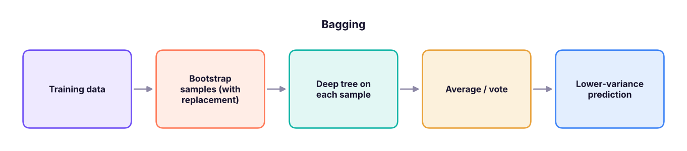
Train each tree on a bootstrap sample (rows drawn with replacement, same size as the data), then average predictions (regression) or vote (classification). Each bootstrap sample leaves out about 37% of rows: the out-of-bag (OOB) rows act as a free validation set.

Bagging: many bootstrap samples, one deep tree each, averaged predictions.

Random forests

A random forest = bagging + a random subset of features considered at each split (max_features). This decorrelates the trees further: a dominant feature cannot sit at the top of every tree.

Python

from sklearn.model_selection import train_test_split, cross_val_score, StratifiedKFold
from sklearn.tree import DecisionTreeClassifier
from sklearn.ensemble import BaggingClassifier, RandomForestClassifier, ExtraTreesClassifier
from sklearn.linear_model import LogisticRegression
from sklearn.metrics import roc_auc_score
tc = pd.read_csv("telecom_churn.csv")
X = pd.get_dummies(tc.drop(columns=["customer_id", "churn", "total_charges"]), drop_first=True).astype(float); y = (tc.churn == "Yes").astype(int)
Xtr, Xte, ytr, yte = train_test_split(X, y, test_size=0.3, stratify=y, random_state=1)
models = {"single deep tree": DecisionTreeClassifier(random_state=0),
          "bagged trees (300)": BaggingClassifier(DecisionTreeClassifier(), n_estimators=300, random_state=0, n_jobs=-1),
          "random forest (300)": RandomForestClassifier(300, random_state=0, n_jobs=-1),
          "random forest, leaf ≥ 20": RandomForestClassifier(300, min_samples_leaf=20, random_state=0, n_jobs=-1),
          "extra trees, leaf ≥ 20": ExtraTreesClassifier(300, min_samples_leaf=20, random_state=0, n_jobs=-1)}
for name, m in models.items():
    m.fit(Xtr, ytr)
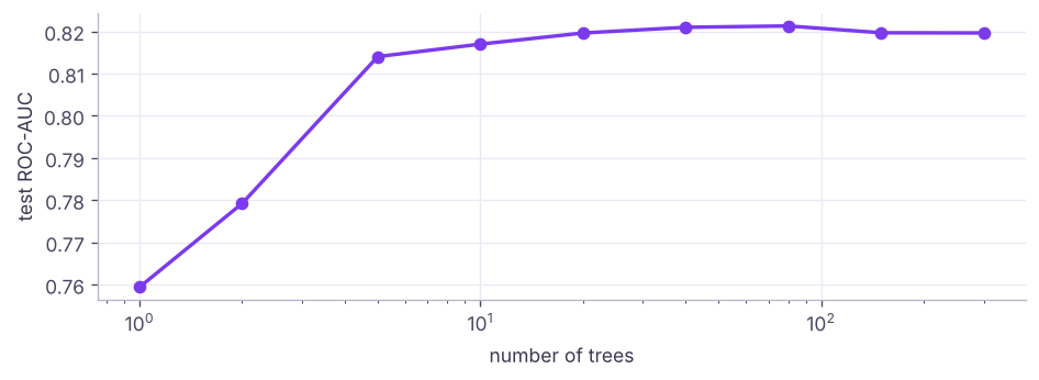
    print(f"{name:26s} train AUC {roc_auc_score(ytr, m.predict_proba(Xtr)[:, 1]):.3f} | test AUC {roc_auc_score(yte, m.predict_proba(Xte)[:, 1]):.3f}")

Output

single deep tree           train AUC 1.000 | test AUC 0.630
bagged trees (300)         train AUC 1.000 | test AUC 0.763
random forest (300)        train AUC 1.000 | test AUC 0.771
random forest, leaf ≥ 20   train AUC 0.847 | test AUC 0.820
extra trees, leaf ≥ 20     train AUC 0.836 | test AUC 0.815

Test AUC as trees are added: performance improves quickly then plateaus; more trees never overfit, they only cost time.

Out-of-bag evaluation

Python

rf = RandomForestClassifier(500, min_samples_leaf=20, oob_score=True, random_state=0, n_jobs=-1).fit(Xtr, ytr)
from sklearn.metrics import roc_auc_score as auc
print(f"OOB accuracy {rf.oob_score_:.3f} | OOB AUC {auc(ytr, rf.oob_decision_function_[:, 1]):.3f} | test AUC {auc(yte, rf.predict_proba(Xte)[:, 1]):.3f}")

Output

OOB accuracy 0.786 | OOB AUC 0.793 | test AUC 0.819

OOB scores approximate test performance without a separate validation set, which is handy for quick tuning.

Key hyperparameters

Parameter	Typical values	Effect
`n_estimators`	200–1,000	More trees = more stable; plateau
`max_features`	`"sqrt"` (classification), 0.3–1.0 (regression)	Lower = more diverse, less correlated trees
`max_depth` / `min_samples_leaf`	None / 1–50	Leaf size smooths probabilities; key for noisy data
`max_samples`	0.5–1.0	Bootstrap sample size (faster, more diverse)
`class_weight`	`"balanced"`, `"balanced_subsample"`	Imbalanced classes
`n_jobs=-1`		Use all CPU cores

Python

from sklearn.model_selection import RandomizedSearchCV
from scipy.stats import randint, uniform
cv = StratifiedKFold(5, shuffle=True, random_state=0)
search = RandomizedSearchCV(RandomForestClassifier(300, random_state=0, n_jobs=-1),
                            {"max_features": uniform(0.1, 0.8), "min_samples_leaf": randint(1, 60), "max_depth": [None, 4, 8, 12]},
                            n_iter=20, cv=cv, scoring="roc_auc", random_state=0).fit(Xtr, ytr)
print({k: (round(float(v), 3) if isinstance(v, float) else v) for k, v in search.best_params_.items()}, f"| CV AUC {search.best_score_:.3f} | test AUC {auc(yte, search.predict_proba(Xte)[:, 1]):.3f}")
lr = LogisticRegression(max_iter=2000).fit(Xtr, ytr); print(f"logistic regression test AUC {auc(yte, lr.predict_proba(Xte)[:, 1]):.3f}")

Output

{'max_depth': 4, 'max_features': 0.37, 'min_samples_leaf': 21} | CV AUC 0.794 | test AUC 0.819
logistic regression test AUC 0.822

On this dataset the relationships are close to additive, so a tuned forest and logistic regression perform similarly. Forests pull ahead when there are strong interactions and thresholds.

Feature importance

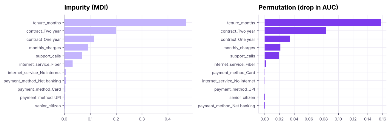
Impurity importance (left) vs permutation importance on the test set (right). Permutation importance measures how much AUC drops when a feature is shuffled.

Python

print(pd.DataFrame({"impurity": imp, "permutation": pi}).sort_values("permutation", ascending=False).round(4).head(6))

Output

                        impurity  permutation
tenure_months             0.4711       0.1575
contract_Two year         0.1996       0.0834
contract_One year         0.1140       0.0339
monthly_charges           0.0925       0.0213
support_calls             0.0683       0.0195
internet_service_Fiber    0.0316       0.0016

Both rank tenure and contract first, but impurity importance (computed on training data) gives continuous features with many possible split points, such as monthly charges, a bigger share; permutation importance on held-out data reflects real predictive value. Neither shows the direction of an effect; use partial dependence or SHAP for that (lesson 27).

Random forest regression

Python

from sklearn.ensemble import RandomForestRegressor
from sklearn.metrics import mean_absolute_error
h = pd.read_csv("house_prices.csv").dropna(subset=["area_sqft"]); h = h[h.price_lakh.between(5, 300)]
Xh = pd.get_dummies(h.drop(columns=["house_id", "price_lakh"]), drop_first=True).astype(float)
a, bq, c, d = train_test_split(Xh, h.price_lakh, test_size=0.2, random_state=0)
rfr = RandomForestRegressor(500, min_samples_leaf=2, max_features=0.6, random_state=0, n_jobs=-1).fit(a, c)
print(f"random forest test MAE {mean_absolute_error(d, rfr.predict(bq)):.2f} lakh | R² {rfr.score(bq, d):.3f}")

Output

random forest test MAE 7.39 lakh | R² 0.912

Voting and stacking

Different model families make different errors, so combining them can help.

Python

from sklearn.ensemble import VotingClassifier, StackingClassifier, HistGradientBoostingClassifier
from sklearn.pipeline import make_pipeline
from sklearn.preprocessing import StandardScaler
from sklearn.neighbors import KNeighborsClassifier
base = [("lr", make_pipeline(StandardScaler(), LogisticRegression(max_iter=2000))), ("rf", RandomForestClassifier(300, min_samples_leaf=20, random_state=0, n_jobs=-1)),
        ("knn", make_pipeline(StandardScaler(), KNeighborsClassifier(75)))]
vote = VotingClassifier(base, voting="soft").fit(Xtr, ytr)
stack = StackingClassifier(base, final_estimator=LogisticRegression(), cv=5).fit(Xtr, ytr)
for name, m in [("soft voting", vote), ("stacking", stack)]: print(f"{name:12s} test AUC {auc(yte, m.predict_proba(Xte)[:, 1]):.3f}")

Output

soft voting  test AUC 0.823
stacking     test AUC 0.824

Soft voting averages predicted probabilities; stacking trains a meta-model on the base models' out-of-fold predictions. Gains are usually small and add complexity; Kaggle winners love them, production teams use them sparingly.

Summary

Key takeaways

Ensembles average diverse models so errors cancel; bagging trains each model on a bootstrap sample.
Random forests add random feature subsets at each split to decorrelate trees; more trees never overfit.
Tune max_features, min_samples_leaf and depth; use OOB scores for quick validation.
Prefer permutation importance on held-out data to impurity importance; neither gives direction.
Voting and stacking combine different model families for small extra gains.

Quick quiz6 questions · tap an answer to check it

1. What is a bootstrap sample?

Answer: A. About 63% of unique rows appear in each.

2. What extra randomness does a random forest add to bagging?

Answer: A. It decorrelates the trees.

3. What happens if you keep adding trees to a random forest?

Answer: A. Unlike boosting rounds.

4. What are out-of-bag rows used for?

Answer: A. No separate validation set needed.

5. Why prefer permutation importance?

Answer: A. Compute it on test or validation data.

6. What does stacking do?

Answer: A. Often a small gain.

ExercisePractice

(1) Fit a random forest on the bank loans data and compare its 5-fold AUC with logistic regression. (2) Plot OOB error vs max_features. (3) Train a RandomForestRegressor on house prices and plot predicted vs actual.

Show solution

Python

b = pd.read_csv("bank_loans.csv").dropna(subset=["default"]); fb = ["age", "ed", "employ", "address", "income", "debtinc", "creddebt", "othdebt"]
for m in (RandomForestClassifier(500, min_samples_leaf=10, random_state=0), make_pipeline(StandardScaler(), LogisticRegression(max_iter=1000))):
    print(type(m).__name__, cross_val_score(m, b[fb], b.default.astype(int), cv=cv, scoring="roc_auc").mean())
for mf in (0.1, 0.3, 0.5, 0.8, 1.0): print(mf, 1 - RandomForestClassifier(300, max_features=mf, oob_score=True, random_state=0).fit(Xtr, ytr).oob_score_)
plt.scatter(d, rfr.predict(bq), s=5); plt.plot([0, 300], [0, 300])

Interview cornerQuestions you may be asked

Q: How does a random forest reduce overfitting compared with a single tree? Each tree sees a different bootstrap sample and random feature subsets, so trees make different errors; averaging them reduces variance while keeping low bias.

Q: Bagging vs boosting? Bagging trains models independently in parallel on bootstrap samples and averages them (reduces variance); boosting trains models sequentially, each correcting the previous errors (reduces bias).

Q: How do you get feature importance from a random forest, and what is the caveat? Impurity-based importance from training splits (biased toward high-cardinality features) or permutation importance on held-out data (more reliable); neither shows the direction of the effect.

Practise more online

Free, trusted places to test yourself on this topic. Links open the original site in a new tab.

← PreviousDecision Trees: Splits, Impurity, Pruning and Interpretable Rules Next →Ensembles II: Gradient Boosting, XGBoost, LightGBM and CatBoost