
A/B Testing and Experimentation: Design, Power, Analysis and Pitfalls
Run product experiments the way data teams at e-commerce and fintech companies do. Choose a metric and guardrails, size the test with power analysis, randomise, analyse conversion and revenue with z-tests, t-tests and bootstrap intervals, check sample-ratio mismatch, avoid peeking and novelty effects, and write the decision memo, using a new-checkout experiment.
- Design an experiment with a hypothesis, primary metric, guardrail metrics and randomisation unit
- Compute the required sample size with power analysis and a minimum detectable effect
- Analyse conversion (two-proportion z-test) and revenue per user (Welch t-test and bootstrap)
- Check sample-ratio mismatch and recognise peeking, novelty and network effects
- Write a launch/no-launch recommendation with uncertainty and business impact
What is an A/B test?
A randomised controlled experiment: users are randomly split into control (A) and treatment (B); the only systematic difference is the change you test, so differences in outcomes are caused by the change (up to chance, which statistics quantifies).

Case. An online store tests a new one-page checkout (B) against the current checkout (A). 4,000 users were split 50/50. Hypothesis: the new checkout increases the purchase conversion rate. Primary metric: conversion = purchasers ÷ users. Secondary: revenue per user, average order value. Guardrails: refund rate, page load time, support tickets.
| Design choice | Good practice |
|---|---|
| Randomisation unit | User (not session or page view), so one person sees one version |
| Split | 50/50 maximises power |
| Duration | At least one full business cycle (1–2 weeks, including weekends); fixed in advance |
| Metric | Defined before launch; one primary metric |
| Population | Who is eligible (new users only? all platforms?) |
Sample size and power
Before launching: how many users do we need to detect the smallest effect worth acting on (the minimum detectable effect, MDE)?
import numpy as np, pandas as pd
from scipy import stats
from statsmodels.stats.power import NormalIndPower
from statsmodels.stats.proportion import proportion_effectsize
base = 0.10
for target in (0.11, 0.12, 0.13):
    h = proportion_effectsize(target, base)                       # Cohen's h
    n = NormalIndPower().solve_power(effect_size=h, alpha=0.05, power=0.8, ratio=1, alternative="two-sided")
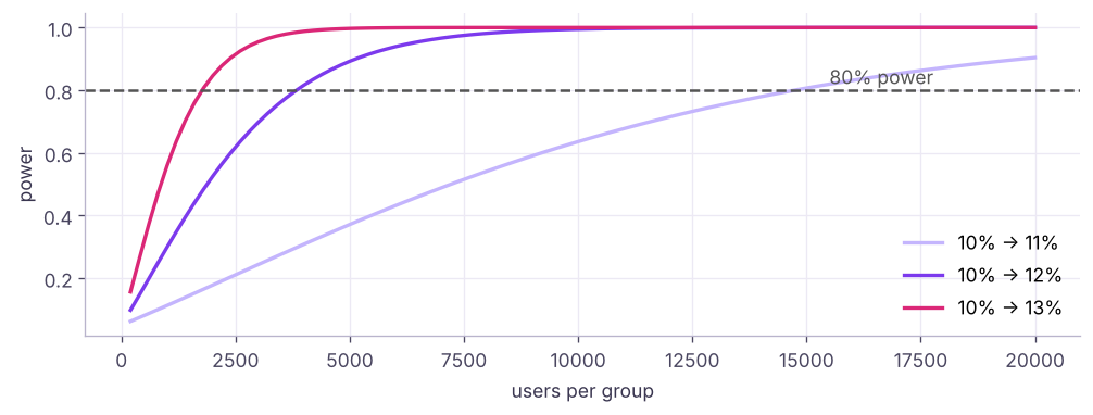
print(f"detect {base:.0%} → {target:.0%} (+{(target - base) / base:.0%} relative): {int(np.ceil(n)):,} users per group")detect 10% → 11% (+10% relative): 14,745 users per group detect 10% → 12% (+20% relative): 3,835 users per group detect 10% → 13% (+30% relative): 1,769 users per group
Small lifts need very large samples. With 2,000 users per group, this test can reliably detect a lift from about 10% to 13%, not smaller ones.
Analysis step 1: sanity checks
ab = pd.read_csv("ab_test.csv")
counts = ab.group.value_counts().sort_index(); print(counts.to_dict())
srm = stats.chisquare(counts.values)                                 # expected 50/50
print(f"sample-ratio mismatch test p = {srm.pvalue:.3f} → {'OK' if srm.pvalue > 0.01 else 'INVESTIGATE: randomisation or logging problem'}")
print("duplicate users:", ab.user_id.duplicated().sum(), "| missing:", ab.isna().sum().sum()){'A_control': 2000, 'B_new_checkout': 2000}
sample-ratio mismatch test p = 1.000 → OK
duplicate users: 0 | missing: 0A sample-ratio mismatch (SRM) (for example 52/48 when you planned 50/50, with p < 0.01) signals a bug in assignment or tracking; do not trust results until it is explained.
Analysis step 2: conversion rate
from statsmodels.stats.proportion import proportions_ztest, confint_proportions_2indep
g = ab.groupby("group").agg(users=("user_id", "size"), buyers=("converted", "sum"))
g["conversion"] = g.buyers / g.users
print(g)
z, p = proportions_ztest(g.buyers.values[::-1], g.users.values[::-1])          # B vs A
lo, hi = confint_proportions_2indep(g.buyers.iloc[1], g.users.iloc[1], g.buyers.iloc[0], g.users.iloc[0], compare="diff")
pa, pb = g.conversion.iloc[0], g.conversion.iloc[1]
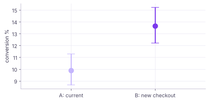
print(f"absolute lift {100 * (pb - pa):.2f} pts (95% CI {100 * lo:.2f} to {100 * hi:.2f}) | relative lift {(pb - pa) / pa:.1%} | z = {z:.2f}, p = {p:.5f}")users buyers conversion group A_control 2000 198 0.0990 B_new_checkout 2000 273 0.1365 absolute lift 3.75 pts (95% CI 1.75 to 5.75) | relative lift 37.9% | z = 3.68, p = 0.00023
Analysis step 3: revenue per user and order value
a, b = ab[ab.group == "A_control"], ab[ab.group == "B_new_checkout"]
for name, col, fa, fb in [("revenue per user", "order_value", a, b), ("average order value (buyers)", "order_value", a[a.converted == 1], b[b.converted == 1])]:
    t = stats.ttest_ind(fb[col], fa[col], equal_var=False)
    print(f"{name:30s} A {fa[col].mean():8.1f} | B {fb[col].mean():8.1f} | diff {fb[col].mean() - fa[col].mean():7.1f} | Welch p = {t.pvalue:.4f}")
rng = np.random.default_rng(0)
boot = [rng.choice(b.order_value.values, len(b)).mean() - rng.choice(a.order_value.values, len(a)).mean() for _ in range(5000)]
print(f"bootstrap 95% CI for revenue-per-user difference: {np.percentile(boot, 2.5):.1f} to {np.percentile(boot, 97.5):.1f}")revenue per user A 137.5 | B 202.8 | diff 65.3 | Welch p = 0.0000 average order value (buyers) A 1389.3 | B 1485.6 | diff 96.4 | Welch p = 0.0082 bootstrap 95% CI for revenue-per-user difference: 35.5 to 94.9
Revenue per user mixes conversion and order size and has many zeros and a long tail; Welch's t-test (thanks to the CLT) and the bootstrap both work at this sample size.
Analysis step 4: business impact
monthly_users = 300_000
extra_buyers = monthly_users * (pb - pa)
extra_rev = monthly_users * (b.order_value.mean() - a.order_value.mean())
print(f"at {monthly_users:,} users/month: about {extra_buyers:,.0f} extra orders and ₹{extra_rev / 1e5:,.1f} lakh extra revenue per month")
print(f"conservative (lower CI bound of conversion lift): {monthly_users * lo:,.0f} extra orders")at 300,000 users/month: about 11,250 extra orders and ₹195.8 lakh extra revenue per month conservative (lower CI bound of conversion lift): 5,263 extra orders
Pitfalls
| Pitfall | What goes wrong | Fix |
|---|---|---|
| Peeking | Checking daily and stopping at the first p < 0.05 inflates false positives to 20–30% | Fix the sample size; or use sequential tests / always-valid p-values |
| Too many metrics | Some will be "significant" by chance | One primary metric; adjust others (lesson 5) |
| Novelty / primacy effects | Users react to change itself, then revert | Run longer; analyse by week |
| SRM | Broken randomisation or logging | Chi-square check before analysis |
| Network effects | Treated users affect control users (marketplaces, social) | Cluster or geo randomisation |
| Simpson's paradox | Mix of segments differs between periods | Randomise; compare within segments |
| Underpowered tests | "No effect" just means "too small a test" | Power analysis first; report CIs |
| HARKing | Choosing the hypothesis after seeing results | Pre-register the plan |
rng = np.random.default_rng(11); false_wins = 0
for sim in range(400):                                         # A/A tests: there is NO real difference
    xa, xb = rng.random(4000) < 0.10, rng.random(4000) < 0.10
    for day in range(1, 15):                                   # peek every "day" (≈285 users per group per day)
        n = day * 285
        if proportions_ztest([xa[:n].sum(), xb[:n].sum()], [n, n])[1] < 0.05: false_wins += 1; break
print(f"stopping at the first significant daily peek: {false_wins / 400:.0%} false positives (should be 5%)")stopping at the first significant daily peek: 20% false positives (should be 5%)
Beyond the classic test
- CUPED / regression adjustment: use pre-experiment behaviour as a covariate to cut variance (and required sample size) by 20–50%.
- Bayesian A/B testing: reports "probability that B beats A" and expected loss; intuitive for stakeholders.
- Multi-armed bandits: shift traffic to the winning variant during the test (good for short campaigns, worse for clean inference).
- Quasi-experiments when you cannot randomise: difference-in-differences, synthetic control, regression discontinuity, propensity matching.
- Platforms: Optimizely, Statsig, GrowthBook, Eppo, LaunchDarkly, Firebase A/B Testing.
The decision memo
Experiment: new one-page checkout, 4,000 users, 50/50, no sample-ratio mismatch. Result: conversion rose from 9.9% to 13.7% (+3.75 points, 95% CI about +1.7 to +5.8; p < 0.001). Revenue per user rose from about ₹138 to ₹203, and buyers' average order value also rose. Guardrails: check refunds, load time and support tickets before rollout. Decision: launch B to all users, with a 5% holdout for four weeks to confirm the effect lasts.
Summary
- Randomisation makes A/B tests causal; define the hypothesis, one primary metric, guardrails and the duration before launch.
- Power analysis sets the sample size for a minimum detectable effect; small lifts need large samples.
- Check sample-ratio mismatch first; analyse conversion with a two-proportion z-test and revenue with Welch's t-test or the bootstrap; report CIs and business impact.
- Avoid peeking, metric fishing and underpowered tests; consider CUPED, Bayesian methods and quasi-experiments where appropriate.
1. Why randomise users into A and B?
2. What does a power analysis give you before the test?
3. The planned split was 50/50 but you observe 53/47 with SRM p < 0.001. What do you do?
4. Why is stopping as soon as p < 0.05 ("peeking") a problem?
5. Which test suits comparing conversion rates of A and B?
6. A test with 300 users per group shows no significant difference. Best conclusion?
(1) Compute the users per group needed to detect a lift from 13.7% to 15% conversion. (2) Analyse average order value among buyers with a Mann-Whitney test as well. (3) Simulate an A/A test 1,000 times with a fixed horizon and confirm about 5% false positives. (4) Draft a one-paragraph memo for the case where the result had been p = 0.20.
Show solution
print(NormalIndPower().solve_power(proportion_effectsize(0.15, 0.137), alpha=0.05, power=0.8))
print(stats.mannwhitneyu(b[b.converted == 1].order_value, a[a.converted == 1].order_value))
fp = np.mean([proportions_ztest([(rng.random(4000) < .1).sum(), (rng.random(4000) < .1).sum()], [4000, 4000])[1] < .05 for _ in range(1000)]); print(fp)
# Memo: "No significant difference (p = 0.20); CI ranges from −x to +y points, so we cannot rule out a meaningful lift. Extend the test to N users or test a bolder change."Q: How would you design an A/B test for a new recommendation widget? State the hypothesis and primary metric (e.g. revenue per user), guardrails (latency, returns), randomise by user, size it with power analysis, run full weeks, check SRM, analyse with CIs, and decide with business impact.
Q: Your test is significant on day 3. Do you stop? No: stopping early inflates false positives and novelty effects can fade; finish the planned duration or use a sequential design.
Q: What if you cannot randomise? Use quasi-experimental methods: difference-in-differences with a comparison group, synthetic control, regression discontinuity or matching, and state the assumptions.
Practise more online
Free, trusted places to test yourself on this topic. Links open the original site in a new tab.