
Gradient Descent: How Models Learn (Built from Scratch in NumPy)
Understand the optimisation engine behind linear regression, logistic regression and neural networks. Cost functions, gradients and the update rule, implementing batch gradient descent for linear regression in NumPy, the learning rate, feature scaling, stochastic and mini-batch variants, convergence checks, and comparison with the closed-form OLS solution and scikit-learn's SGDRegressor.
- Define a cost function (MSE) and explain what its gradient tells us
- Implement batch gradient descent for linear regression with NumPy
- Choose a learning rate and diagnose divergence and slow convergence with cost curves
- Explain why feature scaling speeds up gradient descent
- Compare batch, stochastic and mini-batch gradient descent and use SGDRegressor
Learning = minimising a cost
A model has parameters (weights). Learning means finding the weights that make a cost function as small as possible. For linear regression the usual cost is the mean squared error:

(The ½ simply makes the derivative tidier.) OLS has a formula for the minimum, but most models (logistic regression, neural networks) do not, so we search for it.
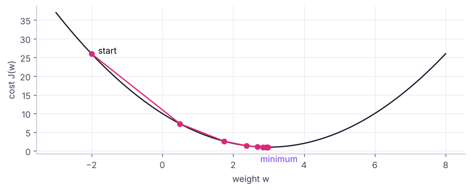
The idea: walk downhill
Imagine standing on a foggy hillside: feel the slope under your feet and step downhill; repeat until the ground is flat. The gradient is the slope; we step in the opposite direction.

α is the learning rate (step size). For linear regression the gradients are:

Implementation in NumPy
import pandas as pd
h = pd.read_csv("house_prices.csv").dropna(subset=["area_sqft"])
pps = h.price_lakh * 1e5 / h.area_sqft; h = h[pps.between(pps.median() / 3, pps.median() * 3)]
feats = ["area_sqft", "bedrooms", "bathrooms", "age_years", "distance_to_center_km"]
X_raw = h[feats].to_numpy(float); y = h.price_lakh.to_numpy(float)
mu, sd = X_raw.mean(axis=0), X_raw.std(axis=0); X = (X_raw - mu) / sd          # standardise features

def gradient_descent(X, y, lr=0.1, epochs=300):
    n, p = X.shape; w, b = np.zeros(p), 0.0; history = []
    for _ in range(epochs):
        y_hat = X @ w + b
        err = y_hat - y
        history.append((err ** 2).mean() / 2)                                   # cost J
        w -= lr * (X.T @ err) / n                                               # gradient step for weights
        b -= lr * err.mean()                                                    # gradient step for bias
    return w, b, history

w, b, hist = gradient_descent(X, y)
print("cost: start", round(hist[0], 1), "→ after 10", round(hist[9], 1), "→ end", round(hist[-1], 2))
print("weights (per 1 sd of each feature):", dict(zip(feats, w.round(2).tolist())), "| bias", round(b, 2))cost: start 3604.0 → after 10 592.8 → end 72.59
weights (per 1 sd of each feature): {'area_sqft': 26.94, 'bedrooms': 1.29, 'bathrooms': -0.48, 'age_years': -3.81, 'distance_to_center_km': -1.12} | bias 79.25Check against the exact OLS solution
X1 = np.c_[np.ones(len(X)), X]
theta = np.linalg.lstsq(X1, y, rcond=None)[0]                                   # closed form (normal equation)
print("OLS bias", theta[0].round(2), "weights", theta[1:].round(2))
print("max difference from gradient descent:", np.abs(theta[1:] - w).max().round(4))
w_orig = w / sd; b_orig = b - (w_orig * mu).sum()                              # convert back to original units
print(f"per sq ft: {w_orig[0]:.4f} lakh (≈ ₹{w_orig[0] * 1e5:,.0f}) | per year of age: {w_orig[3]:.3f} lakh")OLS bias 79.25 weights [26.98 1.16 -0.38 -3.81 -1.12] max difference from gradient descent: 0.1303 per sq ft: 0.0677 lakh (≈ ₹6,769) | per year of age: -0.442 lakh
Gradient descent reached the same answer as the exact formula. The normal equation θ = (XᵀX)⁻¹Xᵀy is fine for a few thousand features, but gradient descent scales to millions of rows and parameters and to models without closed-form solutions.
The learning rate
| Symptom | Cause | Fix |
|---|---|---|
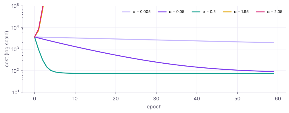
| Cost falls very slowly | α too small | Increase α (×3 steps: 0.001, 0.003, 0.01…) |
| Cost goes up or oscillates, becomes NaN | α too large | Decrease α |
| Cost flattens high | Stuck / underfitting / unscaled features | Scale features, more epochs, better model |
Plot the cost every time: it should go down and flatten.
Why scale features?
best = ((X1 @ theta - y) ** 2).mean() / 2                                     # the lowest possible cost (OLS)
with np.errstate(all="ignore"):
    for name, Xs, lr in [("raw features", X_raw, 1e-7), ("raw features", X_raw, 1e-6), ("standardised", X, 0.1)]:
        _, _, hh = gradient_descent(Xs, y, lr=lr, epochs=300)
        gap = "diverged" if not np.isfinite(hh[-1]) or hh[-1] > 1e6 else f"{100 * (hh[-1] / best - 1):.1f}% above the optimum"
print(f"{name:13s} lr={lr:<6} cost after 300 epochs: {gap}")raw features lr=1e-07 cost after 300 epochs: 14.0% above the optimum raw features lr=1e-06 cost after 300 epochs: 13.3% above the optimum standardised lr=0.1 cost after 300 epochs: 0.0% above the optimum
With raw features, area (hundreds to thousands) and bedrooms (1–5) differ hugely in scale, so the cost surface is a long narrow valley: a learning rate small enough for area is far too small for bedrooms. Standardising makes the valley round, so one learning rate suits all weights.
Batch, stochastic and mini-batch
| Variant | Gradient from | Pros | Cons |
|---|---|---|---|
| Batch GD | All n rows each step | Smooth, exact | Slow for big data |
| Stochastic GD (SGD) | One random row | Fast updates, escapes shallow minima | Noisy |
| Mini-batch GD | 32–1,024 rows | Best of both; GPU friendly | Batch size to tune |
def minibatch_gd(X, y, lr=0.05, epochs=20, batch=32, seed=0):
    rng = np.random.default_rng(seed); n, p = X.shape; w, b = np.zeros(p), 0.0; costs = []
    for _ in range(epochs):
        idx = rng.permutation(n)
        for start in range(0, n, batch):
            j = idx[start:start + batch]; err = X[j] @ w + b - y[j]
            w -= lr * X[j].T @ err / len(j); b -= lr * err.mean()
        costs.append(((X @ w + b - y) ** 2).mean() / 2)
    return w, b, costs
wm, bm, cm = minibatch_gd(X, y)
print("mini-batch cost per epoch:", [round(float(c), 1) for c in cm[:5]], "...", round(float(cm[-1]), 2), "| weights close to OLS:", np.allclose(wm, theta[1:], atol=0.5))mini-batch cost per epoch: [170.3, 79.1, 74.1, 73.5, 73.0] ... 72.62 | weights close to OLS: True
Deep learning uses mini-batch gradient descent with improved optimisers: momentum (keeps velocity), RMSProp and Adam (adaptive learning rates per parameter), plus learning-rate schedules.
scikit-learn: SGDRegressor
from sklearn.linear_model import SGDRegressor, LinearRegression
from sklearn.pipeline import make_pipeline
from sklearn.preprocessing import StandardScaler
from sklearn.model_selection import train_test_split
Xtr, Xte, ytr, yte = train_test_split(h[feats], y, test_size=0.2, random_state=0)
sgd = make_pipeline(StandardScaler(), SGDRegressor(learning_rate="invscaling", eta0=0.01, max_iter=2000, tol=1e-6, random_state=0)).fit(Xtr, ytr)
ols = make_pipeline(StandardScaler(), LinearRegression()).fit(Xtr, ytr)
print(f"test R²: SGDRegressor {sgd.score(Xte, yte):.4f} | LinearRegression {ols.score(Xte, yte):.4f} | SGD epochs used {sgd[-1].n_iter_}")test R²: SGDRegressor 0.8513 | LinearRegression 0.8514 | SGD epochs used 23
SGDRegressor/SGDClassifier also support partial_fit for data that arrives in streams or does not fit in memory, and penalties (L2, L1, elastic net) for regularisation.
Where gradient descent appears
Logistic regression (minimising log loss, lesson 13), neural networks and LLMs (backpropagation computes gradients for billions of weights, lesson 26), gradient boosting (fits each new tree to the gradient of the loss, lesson 19), and matrix factorisation in recommenders.
Summary
- Learning = minimising a cost function; gradient descent repeatedly steps against the gradient: w ← w − α·∂J/∂w.
- For linear regression: gradient = Xᵀ(ŷ − y)/n; it converges to the same solution as OLS.
- The learning rate controls step size: too small is slow, too large diverges; always plot the cost.
- Scale features so one learning rate suits all weights.
- Batch, stochastic and mini-batch variants trade accuracy of each step for speed; Adam and momentum power deep learning.
1. In the update w ← w − α·∂J/∂w, what is α?
2. The cost increases every epoch and becomes NaN. Most likely cause?
3. Why standardise features before gradient descent?
4. What does mini-batch gradient descent use for each update?
5. Gradient descent and the normal equation on the same linear regression should give…
6. Which algorithm fits each new tree to the gradient of the loss?
(1) Add an early-stopping rule: stop when the cost improves by less than 0.001. How many epochs are needed at α = 0.1? (2) Implement gradient descent for a model with only area_sqft and plot the fitted line. (3) Try mini-batch sizes 8, 64 and 512 and compare the final cost after 10 epochs.
Show solution
def gd_early(X, y, lr=0.1, tol=1e-3, max_epochs=10_000):
    n, p = X.shape; w, b = np.zeros(p), 0.0; prev = np.inf
    for e in range(max_epochs):
        err = X @ w + b - y; cost = (err ** 2).mean() / 2
        if prev - cost < tol: return w, b, e
        prev = cost; w -= lr * X.T @ err / n; b -= lr * err.mean()
    return w, b, max_epochs
print(gd_early(X, y)[2])
w1, b1, _ = gradient_descent(X[:, [0]], y)
for bs in (8, 64, 512): print(bs, minibatch_gd(X, y, batch=bs, epochs=10)[2][-1])Q: Explain gradient descent intuitively. Start with random weights, compute how wrong the model is, find the direction that reduces the error fastest (the negative gradient), take a small step, and repeat until the error stops falling.
Q: Batch vs stochastic gradient descent? Batch uses all data per step (stable, slow); stochastic uses one example (fast, noisy); mini-batch is the practical compromise.
Q: Can gradient descent get stuck? For convex costs like linear and logistic regression there is one global minimum. For neural networks it can land in local minima or saddle points; momentum, Adam and random restarts help.
Practise more online
Free, trusted places to test yourself on this topic. Links open the original site in a new tab.