
Decision Trees: Splits, Impurity, Pruning and Interpretable Rules
Learn the model behind random forests and gradient boosting. How trees split data with Gini impurity, entropy and variance reduction, growing and visualising a tree, reading it as business rules, controlling overfitting with depth, minimum leaf size and cost-complexity pruning, regression trees, feature importance and the strengths and weaknesses of single trees.
- Explain recursive binary splitting and compute Gini impurity and entropy by hand
- Train, plot and read a decision tree classifier as IF-THEN rules
- Control overfitting with max_depth, min_samples_leaf and ccp_alpha pruning
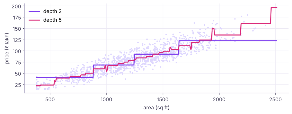
- Build a regression tree and explain its step-shaped predictions
- Describe tree feature importance and the instability of single trees
How a tree decides
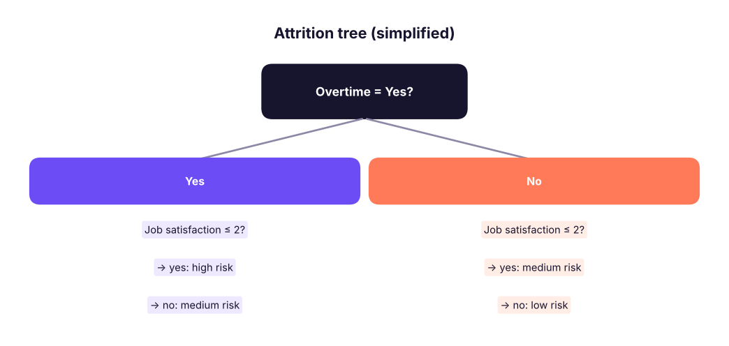
A decision tree asks a sequence of yes/no questions about the features. Each question splits the data into two purer groups; leaves give the prediction (majority class or average value). It is a flowchart learned from data.
Measuring purity
At each node the algorithm tries every feature and threshold and picks the split that most reduces impurity.

import numpy as np, pandas as pd
def gini(p): p = np.asarray(p); return 1 - (p ** 2).sum()
def entropy(p): p = np.asarray([x for x in p if x > 0]); return float(-(p * np.log2(p)).sum()) + 0.0
for dist in ([0.5, 0.5], [0.8, 0.2], [1.0, 0.0]): print(dist, "Gini", round(gini(dist), 3), "| entropy", round(entropy(dist), 3))
hr = pd.read_csv("hr_employees.csv"); hr["left"] = (hr.attrition == "Yes").astype(int)
def split_gain(df, mask):
    parent = gini([1 - df.left.mean(), df.left.mean()])
    l, r = df[mask], df[~mask]
    child = sum(len(s) / len(df) * gini([1 - s.left.mean(), s.left.mean()]) for s in (l, r))
    return parent - child
for name, mask in [("overtime == Yes", hr.overtime == "Yes"), ("job_satisfaction <= 2", hr.job_satisfaction <= 2), ("years_at_company <= 1", hr.years_at_company <= 1), ("department == Sales", hr.department == "Sales")]:
print(f"{name:24s} Gini decrease {split_gain(hr, mask):.4f}")[0.5, 0.5] Gini 0.5 | entropy 1.0 [0.8, 0.2] Gini 0.32 | entropy 0.722 [1.0, 0.0] Gini 0.0 | entropy 0.0 overtime == Yes Gini decrease 0.0094 job_satisfaction <= 2 Gini decrease 0.0086 years_at_company <= 1 Gini decrease 0.0031 department == Sales Gini decrease 0.0015
The split with the largest decrease (information gain) wins; then the process repeats inside each child (recursive binary splitting) until a stopping rule is met. Regression trees use variance (MSE) reduction instead.
Training and reading a tree
from sklearn.tree import DecisionTreeClassifier, export_text, plot_tree
from sklearn.model_selection import train_test_split
from sklearn.metrics import roc_auc_score, accuracy_score
X = pd.get_dummies(hr[["age", "years_at_company", "monthly_income", "job_satisfaction", "distance_from_home_km", "performance_rating", "overtime", "department"]], drop_first=True).astype(float)
y = hr.left
Xtr, Xte, ytr, yte = train_test_split(X, y, test_size=0.3, stratify=y, random_state=0)
small = DecisionTreeClassifier(max_depth=3, min_samples_leaf=40, random_state=0).fit(Xtr, ytr)
print(export_text(small, feature_names=list(X.columns), show_weights=True, decimals=1))
print(f"test AUC {roc_auc_score(yte, small.predict_proba(Xte)[:, 1]):.3f} | accuracy {accuracy_score(yte, small.predict(Xte)):.3f}")|--- overtime_Yes <= 0.5 | |--- job_satisfaction <= 2.5 | | |--- distance_from_home_km <= 15.5 | | | |--- weights: [149.0, 33.0] class: 0 | | |--- distance_from_home_km > 15.5 | | | |--- weights: [104.0, 64.0] class: 0 | |--- job_satisfaction > 2.5 | | |--- distance_from_home_km <= 26.5 | | | |--- weights: [294.0, 41.0] class: 0 | | |--- distance_from_home_km > 26.5 | | | |--- weights: [39.0, 16.0] class: 0 |--- overtime_Yes > 0.5 | |--- years_at_company <= 3.5 | | |--- job_satisfaction <= 2.5 | | | |--- weights: [44.0, 52.0] class: 1 | | |--- job_satisfaction > 2.5 | | | |--- weights: [55.0, 32.0] class: 0 | |--- years_at_company > 3.5 | | |--- monthly_income <= 84708.5 | | | |--- weights: [25.0, 16.0] class: 0 | | |--- monthly_income > 84708.5 | | | |--- weights: [68.0, 18.0] class: 0 test AUC 0.598 | accuracy 0.716
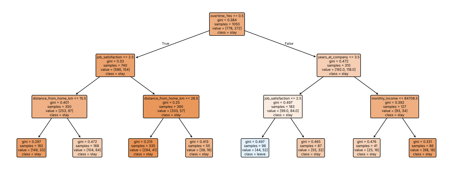
Each path from root to leaf is an IF-THEN rule that managers can read and challenge, which is a big advantage of small trees.
Overfitting and how to stop it
for depth in (1, 2, 3, 5, 8, 12, None):
    m = DecisionTreeClassifier(max_depth=depth, random_state=0).fit(Xtr, ytr)
print(f"max_depth={str(depth):4s} leaves {m.get_n_leaves():4d} | train AUC {roc_auc_score(ytr, m.predict_proba(Xtr)[:, 1]):.3f} | test AUC {roc_auc_score(yte, m.predict_proba(Xte)[:, 1]):.3f}")max_depth=1 leaves 2 | train AUC 0.594 | test AUC 0.552 max_depth=2 leaves 4 | train AUC 0.639 | test AUC 0.591 max_depth=3 leaves 7 | train AUC 0.681 | test AUC 0.598 max_depth=5 leaves 23 | train AUC 0.757 | test AUC 0.571 max_depth=8 leaves 90 | train AUC 0.898 | test AUC 0.597 max_depth=12 leaves 196 | train AUC 0.986 | test AUC 0.579 max_depth=None leaves 255 | train AUC 1.000 | test AUC 0.551
An unrestricted tree keeps splitting until leaves are pure: perfect on training data, poor on new data. Notice also that attrition is hard to predict from these few HR fields (the best test AUC is only about 0.6). That is common with people data: many reasons for leaving (a new offer, a manager, family) are not in the database. A good analyst says so rather than overselling the model.
| Hyperparameter | Effect |
|---|---|
max_depth |
Maximum number of questions on a path |
min_samples_split |
A node needs this many rows to split |
min_samples_leaf |
Every leaf keeps at least this many rows (smooths probabilities) |
max_leaf_nodes |
Cap on the number of leaves |
ccp_alpha |
Cost-complexity pruning: removes branches that add little |
class_weight="balanced" |
Gives the minority class more weight |
Cost-complexity pruning
from sklearn.model_selection import cross_val_score, StratifiedKFold
path = DecisionTreeClassifier(random_state=0).cost_complexity_pruning_path(Xtr, ytr)
alphas = path.ccp_alphas[::max(1, len(path.ccp_alphas) // 25)]
cv = StratifiedKFold(5, shuffle=True, random_state=0)
scores = [cross_val_score(DecisionTreeClassifier(ccp_alpha=a, random_state=0), Xtr, ytr, cv=cv, scoring="roc_auc").mean() for a in alphas]
best_a = alphas[int(np.argmax(scores))]
pruned = DecisionTreeClassifier(ccp_alpha=best_a, random_state=0).fit(Xtr, ytr)
print(f"best ccp_alpha {best_a:.5f} | leaves {pruned.get_n_leaves()} | CV AUC {max(scores):.3f} | test AUC {roc_auc_score(yte, pruned.predict_proba(Xte)[:, 1]):.3f}")best ccp_alpha 0.00320 | leaves 10 | CV AUC 0.607 | test AUC 0.586
Feature importance
imp = pd.Series(pruned.feature_importances_, index=X.columns).sort_values(ascending=False)
print(imp[imp > 0].round(3).to_dict()){'monthly_income': 0.424, 'overtime_Yes': 0.245, 'distance_from_home_km': 0.131, 'job_satisfaction': 0.119, 'years_at_company': 0.08}Importance = total impurity decrease contributed by each feature (normalised to sum to 1). It is quick but biased towards continuous features with many possible split points; check with permutation importance (lesson 27).
Regression trees
from sklearn.metrics import mean_absolute_error
hf = ["area_sqft", "bedrooms", "bathrooms", "age_years", "distance_to_center_km", "parking"]
Htr, Hte, htr, hte = train_test_split(pd.get_dummies(h[hf + ["city"]]).astype(float), h.price_lakh, test_size=0.2, random_state=0)
for d in (3, 6, 10, None):
    t = DecisionTreeRegressor(max_depth=d, min_samples_leaf=5, random_state=0).fit(Htr, htr)
print(f"depth {str(d):4s} test MAE {mean_absolute_error(hte, t.predict(Hte)):.2f} lakh")depth 3 test MAE 10.12 lakh depth 6 test MAE 8.10 lakh depth 10 test MAE 7.62 lakh depth None test MAE 7.64 lakh
Trees cannot extrapolate: a house bigger than any in the training data gets the price of the largest leaf.
Strengths and weaknesses
| Strengths | Weaknesses |
|---|---|
| Easy to explain as rules; visual | Unstable: small data changes give a different tree |
| No scaling needed; handles mixed types | Overfits without limits |
| Captures non-linearity and interactions automatically | Step-shaped, no extrapolation |
| Fast to train and predict | Single trees are usually less accurate than ensembles |
for seed in range(3):
    Xs, _, ys, _ = train_test_split(Xtr, ytr, train_size=0.8, random_state=seed)
    t = DecisionTreeClassifier(max_depth=2, random_state=0).fit(Xs, ys)
print(f"sample {seed}: root split on '{X.columns[t.tree_.feature[0]]}' at {t.tree_.threshold[0]:.1f}, second-level splits on {[X.columns[f] for f in t.tree_.feature[1:] if f >= 0]}")sample 0: root split on 'overtime_Yes' at 0.5, second-level splits on ['distance_from_home_km', 'years_at_company'] sample 1: root split on 'overtime_Yes' at 0.5, second-level splits on ['job_satisfaction', 'years_at_company'] sample 2: root split on 'job_satisfaction' at 2.5, second-level splits on ['distance_from_home_km', 'age']
Instability is exactly what random forests exploit: average many different trees and the noise cancels out (next lesson).
Summary
- Trees split recursively on the feature/threshold that most reduces impurity (Gini, entropy) or variance (regression).
- Small trees are readable IF-THEN rules; unrestricted trees overfit badly.
- Control complexity with max_depth, min_samples_leaf and ccp_alpha pruning, chosen by cross-validation.
- Impurity-based importance is quick but biased; trees need no scaling but cannot extrapolate.
- Single trees are unstable; ensembles (random forests, boosting) fix this.
1. What is the Gini impurity of a node with 50% stay and 50% leave?
2. An unrestricted tree has train AUC 1.0 and test AUC 0.6. Why?
3. Do decision trees need feature scaling?
4. What does min_samples_leaf=40 do?
5. Why can't a regression tree predict prices above the training maximum?
6. Which weakness of single trees do random forests address?
(1) Train a tree on the telecom churn data with depth 3 and write its rules as three bullet points for the retention team. (2) Tune max_depth and min_samples_leaf with GridSearchCV. (3) Compare the test AUC of the pruned tree with logistic regression.
Show solution
tc = pd.read_csv("telecom_churn.csv"); Xc = pd.get_dummies(tc.drop(columns=["customer_id", "churn", "total_charges"]), drop_first=True).astype(float); yc = (tc.churn == "Yes").astype(int)
t3 = DecisionTreeClassifier(max_depth=3, min_samples_leaf=50).fit(Xc, yc); print(export_text(t3, feature_names=list(Xc.columns)))
from sklearn.model_selection import GridSearchCV
g = GridSearchCV(DecisionTreeClassifier(random_state=0), {"max_depth": [2, 3, 4, 5, 6, 8], "min_samples_leaf": [5, 20, 50, 100]}, cv=5, scoring="roc_auc").fit(Xc, yc); print(g.best_params_, g.best_score_)Q: How does a decision tree choose a split? It evaluates candidate thresholds on every feature and picks the one with the largest impurity reduction (Gini or entropy for classification, variance for regression), then repeats recursively.
Q: Gini vs entropy? Both measure impurity and usually give similar trees; Gini is slightly faster, entropy comes from information theory.
Q: How do you prevent a tree from overfitting? Limit depth, require minimum samples per leaf/split, cap leaves, prune with cost-complexity, or use ensembles.
Practise more online
Free, trusted places to test yourself on this topic. Links open the original site in a new tab.