Statistics & Machine Learning · Lesson 19 of 28

Ensembles II: Gradient Boosting, XGBoost, LightGBM and CatBoost

The algorithm family that wins most tabular-data problems. Boosting intuition (AdaBoost to gradient boosting), fitting trees to residuals by hand, learning rate and number of trees, early stopping, scikit-learn's HistGradientBoosting, XGBoost and LightGBM APIs and key hyperparameters, categorical features and CatBoost, and a tuned comparison on churn and house prices.

● ML track (added)✦ XGBoost 3.x · LightGBM 4.x · scikit-learn 1.7+Advanced⏱ 120 min

⬇ Download PDF

By the end of this lesson you can

Explain sequential boosting and how gradient boosting fits trees to residuals (gradients)
Implement a few boosting rounds by hand to see the mechanism
Tune learning rate, number of trees, depth, subsampling and regularisation with early stopping
Use HistGradientBoosting, XGBoost and LightGBM with native categorical handling
Decide when boosting is worth its extra complexity

Datasets used

telecom_churn.csv house_prices.csv

Boosting: learn from mistakes

Bagging trains trees independently and averages them (reduces variance). Boosting trains small trees sequentially: each new tree focuses on what the current ensemble gets wrong (reduces bias).

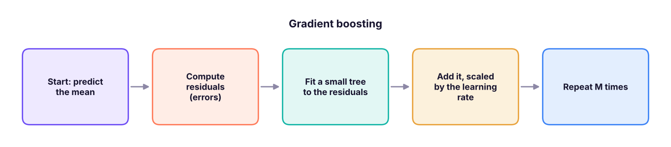
Gradient boosting adds trees one at a time, each correcting the remaining error.

AdaBoost (1995) reweights misclassified rows so the next learner focuses on them.
Gradient boosting (Friedman, 2001) fits each new tree to the negative gradient of the loss; for squared error, that is simply the residual.

F_m(x) = F_{m-1}(x) + \nu \, h_m(x), \qquad h_m \approx -\frac{\partial L(y, F_{m-1})}{\partial F_{m-1}}

Boosting by hand

Python

import numpy as np, pandas as pd
from sklearn.tree import DecisionTreeRegressor
from sklearn.model_selection import train_test_split
from sklearn.metrics import mean_absolute_error
h = pd.read_csv("house_prices.csv").dropna(subset=["area_sqft"]); h = h[h.price_lakh.between(5, 300)]
Xh = pd.get_dummies(h.drop(columns=["house_id", "price_lakh"]), drop_first=True).astype(float); yh = h.price_lakh
Xtr, Xte, ytr, yte = train_test_split(Xh, yh, test_size=0.2, random_state=0)
lr, pred_tr, pred_te = 0.3, np.full(len(ytr), ytr.mean()), np.full(len(yte), ytr.mean())
print(f"round 0 (mean only): test MAE {mean_absolute_error(yte, pred_te):.2f}")
for m in range(1, 31):
    resid = ytr - pred_tr                                      # negative gradient of squared error
    tree = DecisionTreeRegressor(max_depth=3, random_state=0).fit(Xtr, resid)
    pred_tr += lr * tree.predict(Xtr); pred_te += lr * tree.predict(Xte)
    if m in (1, 2, 5, 10, 30): print(f"round {m:2d}: test MAE {mean_absolute_error(yte, pred_te):.2f}")

Output

round 0 (mean only): test MAE 25.00
round  1: test MAE 19.07
round  2: test MAE 15.39
round  5: test MAE 10.61
round 10: test MAE 8.01
round 30: test MAE 6.95

Thirty shallow trees, each correcting the last, beat a single deep tree.

The learning rate and number of trees

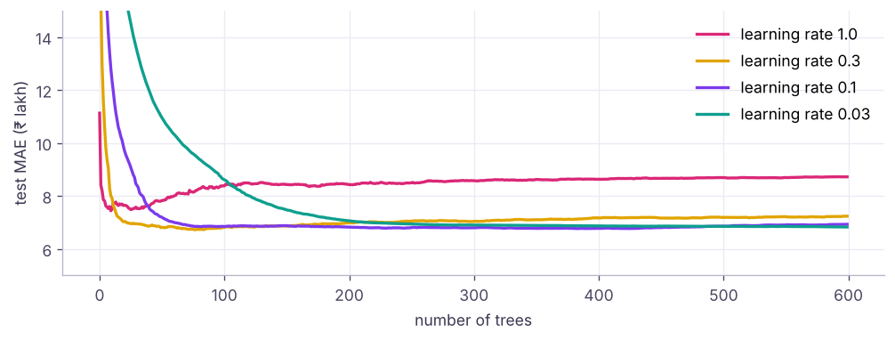
Validation error by boosting round for different learning rates: small rates need more trees but often reach lower error; too many rounds can overfit.

Unlike random forests, boosting can overfit with too many rounds. Use a small learning rate (0.01–0.1) with early stopping on a validation set.

scikit-learn HistGradientBoosting

The fast, modern implementation in scikit-learn (inspired by LightGBM): bins features into histograms, handles missing values and categorical features natively, supports early stopping.

Python

from sklearn.ensemble import HistGradientBoostingClassifier
from sklearn.metrics import roc_auc_score
tc = pd.read_csv("telecom_churn.csv")
Xc = tc.drop(columns=["customer_id", "churn", "total_charges"]); yc = (tc.churn == "Yes").astype(int)
for col in ["contract", "internet_service", "payment_method"]: Xc[col] = Xc[col].astype("category")
Xa, Xb, ya, yb = train_test_split(Xc, yc, test_size=0.3, stratify=yc, random_state=1)
hgb = HistGradientBoostingClassifier(learning_rate=0.05, max_iter=1000, max_depth=None, max_leaf_nodes=15, min_samples_leaf=40, l2_regularization=1.0,
                                     categorical_features="from_dtype", early_stopping=True, validation_fraction=0.15, n_iter_no_change=30, random_state=0).fit(Xa, ya)
print(f"HistGradientBoosting: stopped after {hgb.n_iter_} trees | test AUC {roc_auc_score(yb, hgb.predict_proba(Xb)[:, 1]):.3f}")

Output

HistGradientBoosting: stopped after 87 trees | test AUC 0.806

XGBoost

Python

import xgboost as xgb
Xa_tr, Xa_va, ya_tr, ya_va = train_test_split(Xa, ya, test_size=0.2, stratify=ya, random_state=0)
xg = xgb.XGBClassifier(n_estimators=2000, learning_rate=0.03, max_depth=3, subsample=0.8, colsample_bytree=0.8, min_child_weight=5, reg_lambda=1.0,
                       enable_categorical=True, tree_method="hist", eval_metric="auc", early_stopping_rounds=100, random_state=0)
xg.fit(Xa_tr, ya_tr, eval_set=[(Xa_va, ya_va)], verbose=False)
print(f"XGBoost {xgb.__version__}: best iteration {xg.best_iteration} | test AUC {roc_auc_score(yb, xg.predict_proba(Xb)[:, 1]):.3f}")

Output

XGBoost 3.4.1: best iteration 6 | test AUC 0.806

LightGBM

Python

import lightgbm as lgb
lg = lgb.LGBMClassifier(n_estimators=2000, learning_rate=0.03, num_leaves=15, min_child_samples=40, subsample=0.8, subsample_freq=1, colsample_bytree=0.8, reg_lambda=1.0, random_state=0, verbose=-1)
lg.fit(Xa_tr, ya_tr, eval_set=[(Xa_va, ya_va)], eval_metric="auc", callbacks=[lgb.early_stopping(100, verbose=False)])
print(f"LightGBM {lgb.__version__}: best iteration {lg.best_iteration_} | test AUC {roc_auc_score(yb, lg.predict_proba(Xb)[:, 1]):.3f}")

Output

LightGBM 4.7.0: best iteration 11 | test AUC 0.809

Early stopping chose very few trees for XGBoost and LightGBM here: with 2,000 training rows and a simple signal, validation AUC peaks early. On larger datasets the best iteration is typically in the hundreds or thousands.

LightGBM grows trees leaf-wise (it splits the leaf with the biggest gain), which is fast and accurate on large data; control complexity with num_leaves and min_child_samples. CatBoost uses ordered target statistics for categorical features and symmetric trees; it is often the best choice when there are many high-cardinality categories (pip install catboost).

Key hyperparameters (cheat sheet)

Idea	XGBoost	LightGBM	HistGradientBoosting	Typical
Number of trees	`n_estimators`	`n_estimators`	`max_iter`	Large + early stopping
Step size	`learning_rate`	`learning_rate`	`learning_rate`	0.01–0.1
Tree size	`max_depth`	`num_leaves`, `max_depth`	`max_leaf_nodes`, `max_depth`	depth 3–8 / 15–63 leaves
Leaf size	`min_child_weight`	`min_child_samples`	`min_samples_leaf`	5–100
Row sampling	`subsample`	`subsample` (+ `subsample_freq`)	—	0.6–0.9
Column sampling	`colsample_bytree`	`colsample_bytree`	`max_features`	0.5–0.9
Regularisation	`reg_lambda`, `reg_alpha`, `gamma`	`reg_lambda`, `reg_alpha`	`l2_regularization`
Imbalance	`scale_pos_weight`	`is_unbalance`, `scale_pos_weight`	`class_weight`	ratio of negatives to positives

Tuning recipe: fix a learning rate (0.05), early-stop the number of trees, tune tree size and leaf size, then sampling and regularisation (Optuna works well), and finally lower the learning rate and raise trees for a last bit of accuracy.

Comparison on two problems

Python

from sklearn.model_selection import cross_val_score, StratifiedKFold, KFold
from sklearn.linear_model import LogisticRegression, Ridge
from sklearn.ensemble import RandomForestClassifier, RandomForestRegressor, HistGradientBoostingRegressor
from sklearn.pipeline import make_pipeline
from sklearn.preprocessing import StandardScaler
Xd = pd.get_dummies(Xc, drop_first=True).astype(float)
cv = StratifiedKFold(5, shuffle=True, random_state=0)
cls = {"logistic regression": make_pipeline(StandardScaler(), LogisticRegression(max_iter=2000)), "random forest": RandomForestClassifier(400, min_samples_leaf=20, random_state=0, n_jobs=-1),
       "HistGradientBoosting": HistGradientBoostingClassifier(learning_rate=0.05, max_iter=200, max_leaf_nodes=15, min_samples_leaf=40, random_state=0),
       "XGBoost": xgb.XGBClassifier(n_estimators=300, learning_rate=0.03, max_depth=3, subsample=0.8, colsample_bytree=0.8, random_state=0),
       "LightGBM": lgb.LGBMClassifier(n_estimators=300, learning_rate=0.03, num_leaves=15, min_child_samples=40, random_state=0, verbose=-1)}
print("Churn (5-fold ROC-AUC):")
for n, m in cls.items(): s = cross_val_score(m, Xd, yc, cv=cv, scoring="roc_auc"); print(f"  {n:22s} {s.mean():.3f} ± {s.std():.3f}")
reg = {"ridge": make_pipeline(StandardScaler(), Ridge()), "random forest": RandomForestRegressor(400, min_samples_leaf=2, max_features=0.6, random_state=0, n_jobs=-1),
       "HistGradientBoosting": HistGradientBoostingRegressor(learning_rate=0.05, max_iter=500, random_state=0),
       "XGBoost": xgb.XGBRegressor(n_estimators=600, learning_rate=0.05, max_depth=4, subsample=0.8, colsample_bytree=0.8, random_state=0),
       "LightGBM": lgb.LGBMRegressor(n_estimators=600, learning_rate=0.05, num_leaves=15, random_state=0, verbose=-1)}
print("House prices (5-fold MAE, ₹ lakh):")
for n, m in reg.items(): s = -cross_val_score(m, Xh, yh, cv=KFold(5, shuffle=True, random_state=0), scoring="neg_mean_absolute_error"); print(f"  {n:22s} {s.mean():.2f} ± {s.std():.2f}")

Output

Churn (5-fold ROC-AUC):
  logistic regression    0.812 ± 0.015
  random forest          0.798 ± 0.014
  HistGradientBoosting   0.790 ± 0.016
  XGBoost                0.804 ± 0.012
  LightGBM               0.791 ± 0.010
House prices (5-fold MAE, ₹ lakh):
  ridge                  6.12 ± 0.25
  random forest          6.95 ± 0.36
  HistGradientBoosting   6.79 ± 0.25
  XGBoost                6.48 ± 0.31
  LightGBM               6.73 ± 0.26

Read results honestly: on these clean, mostly additive datasets, linear models are competitive. Boosting's advantage grows with more data, more features, interactions, missing values and messy real-world signals, which is why it dominates tabular competitions and industry credit, fraud, pricing and ranking models.

Summary

Key takeaways

Boosting adds shallow trees sequentially; gradient boosting fits each tree to the negative gradient (residuals for squared error).
The learning rate scales each tree; small rates need more trees; use early stopping because boosting can overfit.
HistGradientBoosting, XGBoost and LightGBM are fast histogram-based implementations with native missing-value and categorical support; CatBoost excels with many categories.
Tune trees (via early stopping), tree/leaf size, sampling and regularisation.
Always compare with simple baselines; boosting shines on large, messy, interaction-rich tabular data.

Quick quiz6 questions · tap an answer to check it

1. How does boosting differ from bagging?

Answer: A. Boosting reduces bias; bagging reduces variance.

2. For squared error, what does each new tree in gradient boosting fit?

Answer: A. Residuals are the negative gradient.

3. What does a smaller learning rate require?

Answer: A. Typical rates are 0.01–0.1.

4. Can gradient boosting overfit by adding too many trees?

Answer: A. Unlike random forests.

5. What does LightGBM's num_leaves control?

Answer: A. Larger = more complex.

6. When is CatBoost particularly useful?

Answer: A. Ordered target statistics handle categories well.

ExercisePractice

(1) Tune LightGBM on the bank loans data with early stopping; compare with logistic regression. (2) Use scale_pos_weight in XGBoost for the churn data and report recall at 0.5. (3) Plot validation AUC against boosting rounds from xg.evals_result().

Show solution

Python

b = pd.read_csv("bank_loans.csv").dropna(subset=["default"]); fb = ["age", "ed", "employ", "address", "income", "debtinc", "creddebt", "othdebt"]
print(cross_val_score(lgb.LGBMClassifier(n_estimators=300, learning_rate=0.03, num_leaves=7, min_child_samples=30, verbose=-1), b[fb], b.default.astype(int), cv=cv, scoring="roc_auc").mean())
from sklearn.metrics import recall_score
w = (ya == 0).sum() / (ya == 1).sum()
xw = xgb.XGBClassifier(n_estimators=300, learning_rate=0.03, max_depth=3, scale_pos_weight=w, enable_categorical=True).fit(Xa, ya)
print(recall_score(yb, xw.predict(Xb)))
plt.plot(xg.evals_result()["validation_0"]["auc"])

Interview cornerQuestions you may be asked

Q: Explain gradient boosting in simple terms. Start with a simple prediction, look at the errors, train a small tree to predict those errors, add a fraction of it, and repeat; the ensemble gradually corrects itself.

Q: XGBoost vs LightGBM vs random forest? Random forests average independent deep trees (robust, little tuning); XGBoost and LightGBM build trees sequentially with regularisation and histogram speed-ups; LightGBM grows leaf-wise and is usually fastest on large data.

Q: How do you prevent overfitting in boosting? Lower learning rate with early stopping, shallow trees, minimum leaf size, row and column subsampling, and L1/L2 regularisation.

Practise more online

Free, trusted places to test yourself on this topic. Links open the original site in a new tab.

← PreviousEnsembles I: Bagging and Random Forests Next →Support Vector Machines and Naive Bayes