
Time-Series Forecasting: Decomposition, Baselines, ETS, ARIMA and ML with Lag Features
Forecast demand properly. Components of a time series (trend, seasonality, noise), decomposition with STL, stationarity and autocorrelation (ADF, ACF/PACF), honest baselines (naive, seasonal naive, moving average), exponential smoothing (Holt-Winters), SARIMA, machine learning with lag and calendar features, backtesting with forecast metrics (MAE, RMSE, MAPE, WAPE), prediction intervals, and a guide to Prophet, statsforecast and foundation models.
- Decompose a series into trend, seasonality and remainder and test stationarity
- Read ACF and PACF plots and difference a series
- Build and evaluate naive, seasonal naive, Holt-Winters and SARIMA forecasts
- Engineer lag, rolling and calendar features and forecast with gradient boosting
- Backtest with a time-ordered holdout, compare models with WAPE/MAPE and report intervals
The data
import pandas as pd, numpy as np, matplotlib.pyplot as plt, warnings
warnings.filterwarnings("ignore")
d = pd.read_csv("daily_sales.csv", parse_dates=["date"]).set_index("date").asfreq("D")
y = d.units_sold
print(y.shape, y.index.min().date(), "to", y.index.max().date(), "| missing days:", y.isna().sum())
print(y.resample("YE").sum().to_dict())
print("mean units by weekday:", y.groupby(y.index.day_name()).mean().round(0).to_dict())(1461,) 2022-01-01 to 2025-12-31 | missing days: 0
{Timestamp('2022-12-31 00:00:00'): 85031, Timestamp('2023-12-31 00:00:00'): 100536, Timestamp('2024-12-31 00:00:00'): 116798, Timestamp('2025-12-31 00:00:00'): 132920}
mean units by weekday: {'Friday': 289.0, 'Monday': 288.0, 'Saturday': 320.0, 'Sunday': 323.0, 'Thursday': 288.0, 'Tuesday': 289.0, 'Wednesday': 287.0}Components of a time series
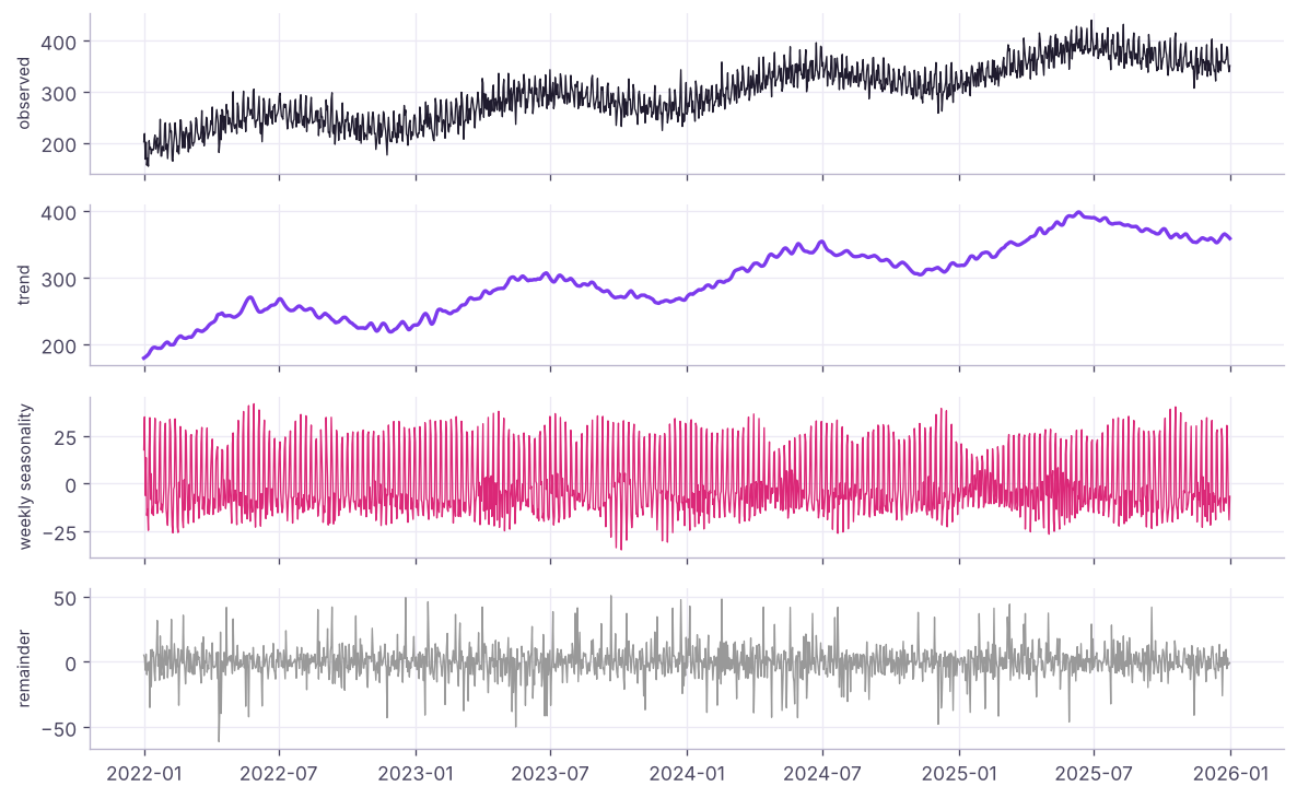
| Component | Meaning | Example |
|---|---|---|
| Trend | Long-term direction | Sales growing about 15% a year |
| Seasonality | Repeating pattern with a fixed period | Weekends higher; December peak; Diwali |
| Cycle | Longer, irregular rises and falls | Economic cycles |
| Remainder / noise | What is left | Random variation, one-off events |
strength_trend = max(0, 1 - res.resid.var() / (res.trend + res.resid).var())
strength_season = max(0, 1 - res.resid.var() / (res.seasonal + res.resid).var())
print(f"strength of trend {strength_trend:.2f} | strength of weekly seasonality {strength_season:.2f} (0 = none, 1 = very strong)")strength of trend 0.95 | strength of weekly seasonality 0.64 (0 = none, 1 = very strong)
Stationarity and autocorrelation
Many classical models (ARIMA) need a stationary series: constant mean and variance over time. Trends and seasonality break that; differencing removes them.
from statsmodels.tsa.stattools import adfuller
for name, s in [("original", y), ("first difference", y.diff()), ("first + weekly difference", y.diff().diff(7))]:
    stat, p = adfuller(s.dropna())[:2]
print(f"{name:26s} ADF p-value {p:.4f} → {'stationary' if p < 0.05 else 'NOT stationary'}")original ADF p-value 0.4455 → NOT stationary first difference ADF p-value 0.0000 → stationary first + weekly difference ADF p-value 0.0000 → stationary
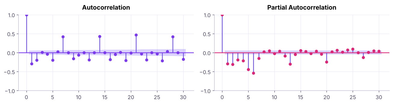
ACF shows correlation with past values at each lag; PACF shows the direct effect of each lag after removing shorter ones. They guide the AR and MA orders of ARIMA models.
Train/test split in time
h = 90                                                     # forecast horizon: the last 90 days
train, test = y.iloc[:-h], y.iloc[-h:]
print(f"train {train.index.min().date()}–{train.index.max().date()} ({len(train)} days) | test {test.index.min().date()}–{test.index.max().date()}")
def metrics(actual, fc):
    e = actual - fc
    return {"MAE": round(float(e.abs().mean()), 1), "RMSE": round(float((e ** 2).mean() ** .5), 1), "MAPE_%": round(float(100 * (e.abs() / actual).mean()), 2),
            "WAPE_%": round(float(100 * e.abs().sum() / actual.sum()), 2), "bias_%": round(float(100 * -e.sum() / actual.sum()), 2)}      # bias > 0 = over-forecast
results, forecasts = {}, {}train 2022-01-01–2025-10-02 (1371 days) | test 2025-10-03–2025-12-31
Never shuffle time series: always train on the past and test on the future.
| Metric | Use |
|---|---|
| MAE / RMSE | Error in units; RMSE punishes big misses |
| MAPE | Percentage error; breaks when actuals are near zero |
| WAPE | Total absolute error ÷ total actuals; robust, preferred in retail |
| Bias | Systematic over- or under-forecasting (stock-outs vs excess inventory) |
Baselines
forecasts["naive"] = pd.Series(train.iloc[-1], index=test.index)
forecasts["seasonal naive (last week)"] = pd.Series(np.tile(train.iloc[-7:].values, h // 7 + 1)[:h], index=test.index)
forecasts["moving average (28 days)"] = pd.Series(train.iloc[-28:].mean(), index=test.index)
for k, f in forecasts.items(): results[k] = metrics(test, f)
print(pd.DataFrame(results).T)MAE RMSE MAPE_% WAPE_% bias_% naive 19.1 22.4 5.36 5.31 1.79 seasonal naive (last week) 14.9 19.1 4.23 4.14 2.35 moving average (28 days) 20.9 23.9 5.92 5.81 2.96
The seasonal naive forecast ("same as last week") is the baseline every serious model must beat.
Exponential smoothing (Holt-Winters / ETS)
ETS forecasts are weighted averages of past observations, with weights decaying exponentially, plus components for level, trend and seasonality.
from statsmodels.tsa.holtwinters import ExponentialSmoothing
ets = ExponentialSmoothing(train, trend="add", damped_trend=True, seasonal="mul", seasonal_periods=7).fit(optimized=True)
forecasts["Holt-Winters (ETS)"] = ets.forecast(h); results["Holt-Winters (ETS)"] = metrics(test, forecasts["Holt-Winters (ETS)"])
print({k: round(float(v), 3) for k, v in ets.params.items() if k in ("smoothing_level", "smoothing_trend", "smoothing_seasonal", "damping_trend")})
print(results["Holt-Winters (ETS)"]){'smoothing_level': 0.054, 'smoothing_trend': 0.054, 'smoothing_seasonal': 0.036, 'damping_trend': 0.989}
{'MAE': 10.4, 'RMSE': 12.8, 'MAPE_%': 2.92, 'WAPE_%': 2.88, 'bias_%': 0.34}SARIMA
ARIMA(p, d, q) combines autoregression (p past values), differencing (d) and moving average of past errors (q). SARIMA adds seasonal terms (P, D, Q, s).
from statsmodels.tsa.statespace.sarimax import SARIMAX
sar = SARIMAX(train, order=(1, 1, 1), seasonal_order=(1, 1, 1, 7)).fit(disp=False)
fc = sar.get_forecast(h); forecasts["SARIMA(1,1,1)(1,1,1,7)"] = fc.predicted_mean; ci = fc.conf_int(alpha=0.05)
results["SARIMA(1,1,1)(1,1,1,7)"] = metrics(test, forecasts["SARIMA(1,1,1)(1,1,1,7)"])
inside = ((test >= ci.iloc[:, 0]) & (test <= ci.iloc[:, 1])).mean()
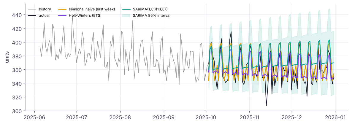
print(f"AIC {sar.aic:.0f} | {results['SARIMA(1,1,1)(1,1,1,7)']} | 95% interval covers {inside:.0%} of test days")AIC 11298 | {'MAE': 16.9, 'RMSE': 20.2, 'MAPE_%': 4.82, 'WAPE_%': 4.69, 'bias_%': 4.06} | 95% interval covers 96% of test daysUse pmdarima.auto_arima or statsforecast.AutoARIMA to search orders automatically by AIC.
Machine learning with lag features
Turn forecasting into regression: predict today's value from lags (same day last week), rolling statistics and calendar features.
import lightgbm as lgb
def make_features(s):
    f = pd.DataFrame(index=s.index)
    f["dow"] = s.index.dayofweek; f["month"] = s.index.month; f["dayofyear"] = s.index.dayofyear; f["t"] = np.arange(len(s))
    for lag in (7, 14, 21, 28, 364): f[f"lag_{lag}"] = s.shift(lag)
    f["roll_mean_28_lag7"] = s.shift(7).rolling(28).mean(); f["roll_std_28_lag7"] = s.shift(7).rolling(28).std()
    return f
F = make_features(y)
Xtr, ytr = F.loc[train.index].dropna(), train.loc[F.loc[train.index].dropna().index]
model = lgb.LGBMRegressor(n_estimators=600, learning_rate=0.03, num_leaves=15, min_child_samples=20, verbose=-1, random_state=0, linear_tree=True).fit(Xtr, ytr)
Lags are at least 7 days, so the model can forecast up to a week ahead without knowing the in-between values. For a 90-day horizon we forecast recursively: predict a week, feed predictions back as lags, repeat.
hist = train.copy()
for day in test.index:
    s = pd.concat([hist, pd.Series([np.nan], index=[day])])
    hist.loc[day] = model.predict(make_features(s).iloc[[-1]])[0]
forecasts["LightGBM (lags, recursive)"] = hist.loc[test.index]; results["LightGBM (lags, recursive)"] = metrics(test, forecasts["LightGBM (lags, recursive)"])
print(pd.DataFrame(results).T.sort_values("WAPE_%"))MAE RMSE MAPE_% WAPE_% bias_% Holt-Winters (ETS) 10.4 12.8 2.92 2.88 0.34 seasonal naive (last week) 14.9 19.1 4.23 4.14 2.35 SARIMA(1,1,1)(1,1,1,7) 16.9 20.2 4.82 4.69 4.06 naive 19.1 22.4 5.36 5.31 1.79 moving average (28 days) 20.9 23.9 5.92 5.81 2.96 LightGBM (lags, recursive) 21.1 27.4 6.01 5.86 4.53
Holt-Winters wins clearly here (WAPE under 3%, almost no bias), while this LightGBM set-up does worse than the seasonal naive baseline. Two reasons: errors accumulate when 90 days are forecast recursively from the model's own predictions, and with a single, smooth series there is little for a tree model to learn that ETS does not already capture. ML models shine with many related series and external drivers (prices, promotions, weather, holidays). The lesson: always benchmark against simple models.
Backtesting
One holdout can be lucky. Rolling-origin backtests repeat the exercise from several start dates.
origins = [pd.Timestamp("2025-03-31"), pd.Timestamp("2025-06-30"), pd.Timestamp("2025-09-30")]
rows = []
for o in origins:
    tr, te = y.loc[:o], y.loc[o + pd.Timedelta(days=1): o + pd.Timedelta(days=28)]
    snaive = pd.Series(np.tile(tr.iloc[-7:].values, 5)[:len(te)], index=te.index)
    ets_o = ExponentialSmoothing(tr, trend="add", damped_trend=True, seasonal="mul", seasonal_periods=7).fit().forecast(len(te))
    rows.append({"origin": o.date(), "seasonal naive WAPE": metrics(te, snaive)["WAPE_%"], "ETS WAPE": metrics(te, ets_o)["WAPE_%"]})
bt = pd.DataFrame(rows); print(bt.to_string(index=False)); print("mean:", bt.drop(columns="origin").mean().round(2).to_dict()) origin seasonal naive WAPE ETS WAPE
2025-03-31 4.44 3.21
2025-06-30 4.04 4.23
2025-09-30 3.08 2.92
mean: {'seasonal naive WAPE': 3.85, 'ETS WAPE': 3.45}Tools and practice
| Tool | Strength |
|---|---|
| statsmodels | ETS, SARIMA(X), decomposition, diagnostics |
| statsforecast (Nixtla) | Very fast AutoARIMA/AutoETS for thousands of series |
| Prophet | Trend + seasonality + holidays with intuitive settings |
| LightGBM / XGBoost with lags | Many related series, external drivers (price, promotions, weather) |
| Deep learning (N-BEATS, TFT) and foundation models (TimeGPT, Chronos, TimesFM) | Large collections of series, zero-shot forecasts |
| Excel / Power BI forecast | Quick ETS forecasts for business users |
Practical tips: forecast at the level decisions are made (store × product × week), add known future drivers (holidays, promotions, prices), forecast intervals not just points, monitor bias, and combine forecasts (an average of ETS and ML often beats both).
Summary
- Decompose series into trend, seasonality and remainder (STL); difference to make them stationary (ADF test); read ACF/PACF.
- Split by time; evaluate with MAE, RMSE, MAPE, WAPE and bias; always beat the seasonal naive baseline.
- Holt-Winters (ETS) models level, trend and seasonality; SARIMA models autocorrelation and seasonal differences, with prediction intervals.
- Gradient boosting with lag, rolling and calendar features is a strong approach, especially with many series and external drivers; forecast recursively for long horizons.
- Backtest from several origins and choose by business metrics.
1. Which baseline must every daily retail forecast beat?
2. What does differencing do?
3. Why is WAPE often preferred to MAPE?
4. In SARIMA(1,1,1)(1,1,1,7), what is 7?
5. Why shouldn't you shuffle data when validating forecasts?
6. A lag-7 feature allows a model to forecast how many days ahead directly?
(1) Aggregate to weekly totals and forecast 12 weeks with Holt-Winters (seasonal period 52 needs 2+ years of data). (2) Add a Diwali/holiday flag feature to the LightGBM model. (3) Average the ETS and SARIMA forecasts: does the WAPE improve?
Show solution
wk = y.resample("W-SUN").sum().iloc[1:-1]
ewk = ExponentialSmoothing(wk.iloc[:-12], trend="add", seasonal="add", seasonal_periods=52).fit().forecast(12)
print(metrics(wk.iloc[-12:], ewk))
combo = (forecasts["Holt-Winters (ETS)"] + forecasts["SARIMA(1,1,1)(1,1,1,7)"]) / 2; print(metrics(test, combo))
diwali = pd.to_datetime(["2022-10-24", "2023-11-12", "2024-11-01", "2025-10-20"])
F["festive"] = [int(any(abs((d - x).days) <= 3 for x in diwali)) for d in F.index]Q: How would you forecast sales for 5,000 products in 200 stores? Hierarchical, automated approach: a global gradient-boosting model with lags, calendar, price and promotion features (or fast AutoETS per series), backtesting by store-product, reconciliation across levels, and monitoring of bias and accuracy.
Q: What is stationarity and why does it matter? Constant statistical properties over time; ARIMA-type models assume it, so we difference or transform the series first.
Q: How do you evaluate a forecasting model? Time-ordered holdout or rolling-origin backtests with MAE/WAPE and bias, comparison with a seasonal naive baseline, and checking prediction-interval coverage.
Practise more online
Free, trusted places to test yourself on this topic. Links open the original site in a new tab.