
Explainable AI and MLOps: SHAP, Fairness, Deployment, Monitoring and Responsible ML
Make models trustworthy and useful in production. Global and local explanations (permutation importance, partial dependence, SHAP), fairness checks across groups, packaging a pipeline, serving predictions with FastAPI, batch scoring, experiment tracking with MLflow, monitoring data drift and performance, model cards, and the regulations and responsible-AI practices that apply in India and globally.
- Explain a model globally with permutation importance and partial dependence
- Explain individual predictions with SHAP values and communicate them
- Check performance and error rates across groups for fairness
- Package, serve and batch-score a model, and track experiments
- Monitor drift and performance after deployment and document models with model cards
Why explainability?
Stakeholders ask "why did the model say this?". Regulators require explanations for credit and insurance decisions; data scientists need explanations to debug leakage and bias.
import pandas as pd, numpy as np, warnings
warnings.filterwarnings("ignore")
from sklearn.model_selection import train_test_split
from sklearn.ensemble import HistGradientBoostingClassifier
from sklearn.metrics import roc_auc_score
tc = pd.read_csv("telecom_churn.csv")
X = pd.get_dummies(tc.drop(columns=["customer_id", "churn", "total_charges"]), drop_first=True).astype(float); y = (tc.churn == "Yes").astype(int)
Xtr, Xte, ytr, yte = train_test_split(X, y, test_size=0.3, stratify=y, random_state=1)
model = HistGradientBoostingClassifier(max_iter=200, learning_rate=0.05, max_leaf_nodes=15, min_samples_leaf=40, random_state=0).fit(Xtr, ytr)
print(f"test AUC {roc_auc_score(yte, model.predict_proba(Xte)[:, 1]):.3f} | features: {list(X.columns)}")test AUC 0.801 | features: ['senior_citizen', 'tenure_months', 'monthly_charges', 'support_calls', 'contract_One year', 'contract_Two year', 'internet_service_Fiber', 'internet_service_No internet', 'payment_method_Card', 'payment_method_Net banking', 'payment_method_UPI']
| Scope | Question | Methods |
|---|---|---|
| Global | Which features matter overall, and how? | Permutation importance, partial dependence, SHAP summary |
| Local | Why this prediction for this customer? | SHAP values, LIME, counterfactuals |
| Interpretable by design | Can the model itself be read? | Linear/logistic models, small trees, scorecards, EBMs |
Global: permutation importance
from sklearn.inspection import permutation_importance
pi = permutation_importance(model, Xte, yte, scoring="roc_auc", n_repeats=15, random_state=0)
imp = pd.DataFrame({"mean_AUC_drop": pi.importances_mean, "std": pi.importances_std}, index=X.columns).sort_values("mean_AUC_drop", ascending=False)
print(imp.round(4))mean_AUC_drop std tenure_months 0.1541 0.0142 contract_Two year 0.0783 0.0121 contract_One year 0.0420 0.0102 monthly_charges 0.0352 0.0123 support_calls 0.0306 0.0071 internet_service_Fiber 0.0026 0.0021 internet_service_No internet 0.0020 0.0016 senior_citizen 0.0006 0.0010 payment_method_UPI 0.0006 0.0012 payment_method_Net banking 0.0005 0.0023 payment_method_Card 0.0001 0.0013
Shuffle one column in the test set and measure how much the score drops: model-agnostic and honest about held-out performance. Correlated features share credit, so treat their importances together.
Global: partial dependence
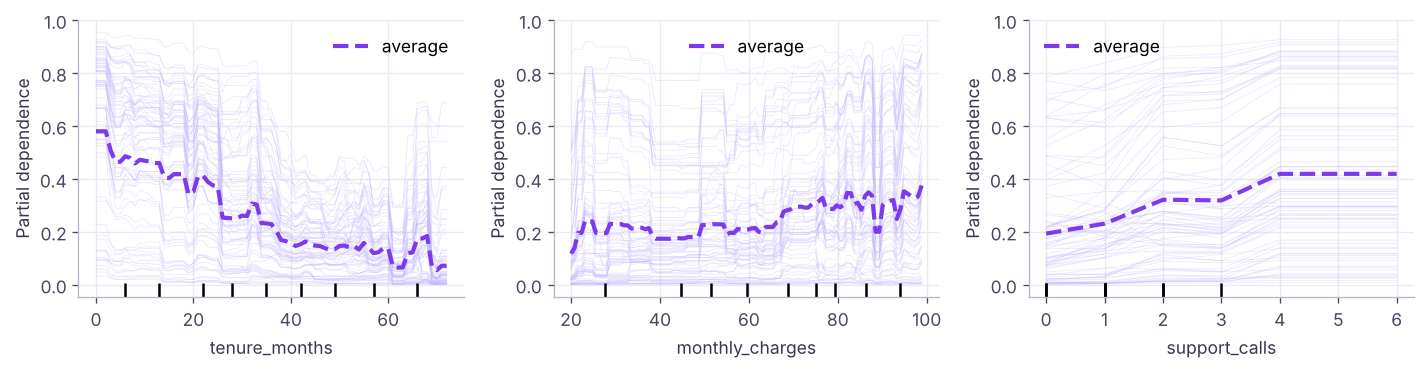
Churn falls steeply in the first two years of tenure, rises with monthly charges and with each extra support call: consistent with the EDA, which builds trust in the model.
Local: SHAP values
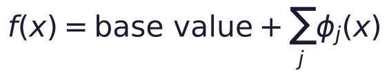
SHAP (SHapley Additive exPlanations) splits each prediction into contributions from each feature, based on Shapley values from cooperative game theory:
import shap
explainer = shap.Explainer(model.predict_proba, shap.maskers.Independent(Xtr, max_samples=200), feature_names=list(X.columns))
sample = Xte.iloc[:200]
sv = explainer(sample, silent=True)[..., 1]                                  # contributions to P(churn)
print("SHAP values shape:", sv.values.shape, "| base value (average prediction):", round(float(sv.base_values[0]), 3))
mean_abs = pd.Series(np.abs(sv.values).mean(0), index=X.columns).sort_values(ascending=False)
print("mean |SHAP| (global importance):", mean_abs.round(4).head(6).to_dict())SHAP values shape: (200, 11) | base value (average prediction): 0.245
mean |SHAP| (global importance): {'tenure_months': 0.1417, 'contract_Two year': 0.0715, 'contract_One year': 0.0702, 'support_calls': 0.0555, 'monthly_charges': 0.0552, 'internet_service_Fiber': 0.012}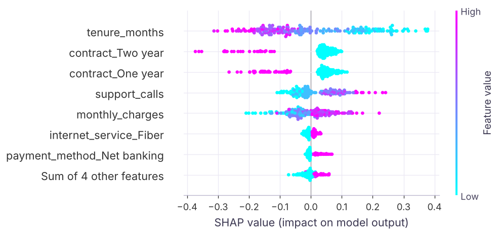
Explaining one customer
probs = model.predict_proba(sample)[:, 1]; i = int(np.argmax(probs))
row = pd.DataFrame({"value": sample.iloc[i], "shap": sv.values[i]}).sort_values("shap", key=abs, ascending=False)
print(f"customer {tc.loc[sample.index[i], 'customer_id']}: P(churn) = {probs[i]:.2f} = base {sv.base_values[i]:.2f} + contributions:")
print(row.head(6).round(3))
def reason(f, v):
    name = f.replace("_", " ")
    if X[f].isin([0, 1]).all() and "_" in f and f not in ("senior_citizen",): return f"not on '{f.split('_', 1)[1]}' {f.split('_')[0]}" if v == 0 else f"{f.split('_', 1)[1]} {f.split('_')[0]}"
    return f"{name} = {v:g}"
reasons = [reason(f, v) for f, v in row[row.shap > 0].value.head(3).items()]
print("Top reasons for the retention agent:", "; ".join(reasons))customer T00216: P(churn) = 0.90 = base 0.25 + contributions:
value shap
tenure_months 4.00 0.261
support_calls 5.00 0.188
contract_Two year 0.00 0.097
monthly_charges 76.23 0.064
contract_One year 0.00 0.050
payment_method_Card 0.00 -0.010
Top reasons for the retention agent: tenure months = 4; support calls = 5; not on 'Two year' contract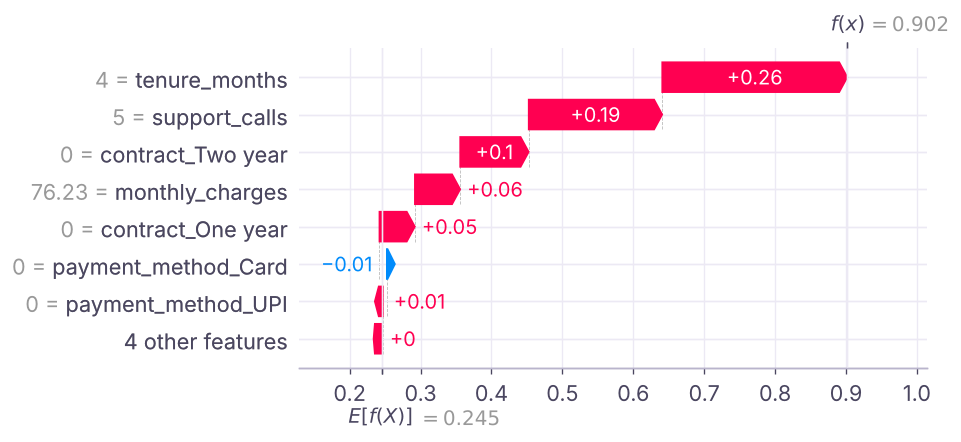
shap.TreeExplainer is much faster for tree models (XGBoost, LightGBM, random forests); shap.LinearExplainer for linear models. Explanations describe the model, not causal effects in the real world.
Fairness checks
A model can be accurate overall and still treat groups differently. Check metrics by group for sensitive attributes (gender, age, region, language).
from sklearn.metrics import recall_score, precision_score
t = 0.4; pred = model.predict_proba(Xte)[:, 1] >= t
grp = np.where(Xte.senior_citizen == 1, "senior", "non-senior")
rows = []
for g in ["non-senior", "senior"]:
    m = grp == g
    rows.append({"group": g, "n": int(m.sum()), "actual churn": round(yte[m].mean(), 3), "flagged rate": round(pred[m].mean(), 3), "recall": round(recall_score(yte[m], pred[m]), 3), "precision": round(precision_score(yte[m], pred[m]), 3), "AUC": round(roc_auc_score(yte[m], model.predict_proba(Xte[m])[:, 1]), 3)})
print(pd.DataFrame(rows).to_string(index=False)) group n actual churn flagged rate recall precision AUC
non-senior 758 0.245 0.243 0.538 0.543 0.806
senior 142 0.324 0.254 0.565 0.722 0.783| Fairness notion | Asks | Note |
|---|---|---|
| Demographic parity | Same positive (flag) rate across groups? | Ignores real differences in base rates |
| Equal opportunity | Same recall (true-positive rate)? | Common for benefits such as retention offers |
| Equalised odds | Same TPR and FPR? | Stricter |
| Calibration within groups | Does 30% mean 30% in every group? | Important for risk scores |
The definitions can conflict; choose with domain experts and legal advice, document the choice, and remove proxies for protected attributes where required. Tools: Fairlearn, AIF360.
From notebook to production

1. Package the pipeline and track the experiment
import joblib, json, sklearn, os, datetime
os.makedirs("artifacts", exist_ok=True)
joblib.dump(model, "artifacts/churn_model.joblib")
card = {"model": "churn HistGradientBoosting", "trained": datetime.date(2026, 1, 15).isoformat(), "sklearn": sklearn.__version__, "features": list(X.columns),
        "test_auc": round(roc_auc_score(yte, model.predict_proba(Xte)[:, 1]), 3), "threshold": t, "intended_use": "monthly retention targeting; not for pricing or credit decisions",
        "training_data": "telecom_churn.csv, 3,000 customers, churn rate 25.7%", "limitations": "no usage or complaint text features; senior customers under-represented"}
json.dump(card, open("artifacts/model_card.json", "w"), indent=2)
print(sorted(os.listdir("artifacts")), "|", json.load(open("artifacts/model_card.json"))["intended_use"])['churn_model.joblib', 'model_card.json'] | monthly retention targeting; not for pricing or credit decisions
# Experiment tracking with MLflow (pip install mlflow; run `mlflow ui` to browse)
import mlflow
with mlflow.start_run(run_name="hgb_v3"):
    mlflow.log_params({"learning_rate": 0.05, "max_leaf_nodes": 15})
    mlflow.log_metric("test_auc", 0.80)
    mlflow.sklearn.log_model(model, name="churn_model", registered_model_name="churn")
2. Serve predictions with an API
from fastapi import FastAPI
from fastapi.testclient import TestClient
from pydantic import BaseModel, Field
app = FastAPI(title="Churn scoring API")
mdl = joblib.load("artifacts/churn_model.joblib"); FEATS = card["features"]
class Customer(BaseModel):
    senior_citizen: int = Field(ge=0, le=1); tenure_months: int = Field(ge=0); monthly_charges: float = Field(gt=0); support_calls: int = Field(ge=0)
    contract: str; internet_service: str; payment_method: str
@app.post("/predict")
def predict(c: Customer):
    row = pd.get_dummies(pd.DataFrame([c.model_dump()])).reindex(columns=FEATS, fill_value=0).astype(float)
    p = float(mdl.predict_proba(row)[0, 1])
    return {"churn_probability": round(p, 3), "flag_for_retention": p >= card["threshold"], "model_version": card["trained"]}
client = TestClient(app)
r = client.post("/predict", json={"senior_citizen": 0, "tenure_months": 2, "monthly_charges": 99.5, "support_calls": 4, "contract": "Month-to-month", "internet_service": "Fiber", "payment_method": "UPI"})
print(r.status_code, r.json())
print(client.post("/predict", json={"senior_citizen": 3, "tenure_months": -1, "monthly_charges": 50, "support_calls": 0, "contract": "x", "internet_service": "y", "payment_method": "z"}).status_code, "(invalid input rejected)")200 {'churn_probability': 0.942, 'flag_for_retention': True, 'model_version': '2026-01-15'}
422 (invalid input rejected)Run it for real with uvicorn app:app --reload, containerise with Docker, and deploy to a cloud service (AWS SageMaker, Azure ML, Google Vertex AI, Cloud Run, Render). Many business models do not need an API at all: a nightly batch job that writes scores to a database table feeding the CRM or a Power BI dashboard is simpler and cheaper.
3. Monitor
from scipy.stats import ks_2samp
def psi(expected, actual, bins=10):
    edges = np.unique(np.quantile(expected, np.linspace(0, 1, bins + 1))); edges[0], edges[-1] = -np.inf, np.inf
    e = np.histogram(expected, edges)[0] / len(expected); a = np.histogram(actual, edges)[0] / len(actual)
    e, a = np.clip(e, 1e-4, None), np.clip(a, 1e-4, None); return float(((a - e) * np.log(a / e)).sum())
rng = np.random.default_rng(0)
new_month = Xte.copy(); new_month["monthly_charges"] = new_month.monthly_charges * 1.12 + rng.normal(0, 3, len(new_month))   # simulated price increase
for col in ["tenure_months", "monthly_charges", "support_calls"]:
    print(f"{col:16s} PSI {psi(Xtr[col], new_month[col]):.3f} | KS p-value {ks_2samp(Xtr[col], new_month[col]).pvalue:.3g}")
print("PSI guide: < 0.1 stable | 0.1–0.25 watch | > 0.25 significant shift → investigate / retrain")tenure_months PSI 0.022 | KS p-value 0.294 monthly_charges PSI 0.538 | KS p-value 1.36e-11 support_calls PSI 0.004 | KS p-value 0.808 PSI guide: < 0.1 stable | 0.1–0.25 watch | > 0.25 significant shift → investigate / retrain
| Monitor | Why |
|---|---|
| Input drift (PSI, KS tests) | The population changed (new pricing, new channel) |
| Prediction drift | Score distribution shifts |
| Performance (once labels arrive) | AUC, recall at threshold, calibration |
| Business KPIs | Retention rate, campaign ROI (via A/B holdouts) |
| Data quality | Missing values, schema changes, pipeline failures |
Tools: Evidently, WhyLabs, Arize, cloud-native monitors; schedule retraining or trigger it when drift or decay crosses thresholds.
Responsible AI and regulation
- Privacy: India's Digital Personal Data Protection Act 2023 (and its 2025 rules), GDPR in Europe: lawful purpose, consent, data minimisation and the right to erasure.
- Credit and lending: RBI guidelines on digital lending expect transparency on decisions; lenders must be able to explain adverse decisions.
- EU AI Act (phased in from 2025–2027): risk tiers; high-risk systems (credit scoring, hiring) need risk management, documentation, human oversight and logging.
- Practice: model cards and datasheets, human review for high-impact decisions, bias testing before launch, red-teaming GenAI systems, and an incident process.
import shutil; shutil.rmtree("artifacts")Summary
- Global explanations: permutation importance (held-out) and partial dependence; local explanations: SHAP values that sum from the base value to the prediction.
- Check metrics by group (recall, precision, calibration) and choose a fairness definition with domain experts.
- Production means a versioned pipeline, model card, experiment tracking, serving (batch or API with input validation) and monitoring.
- Monitor input drift (PSI/KS), prediction drift, performance and business KPIs; retrain on a schedule or on triggers.
- Follow privacy and AI regulations (DPDP Act, RBI, EU AI Act) and keep humans in the loop for high-impact decisions.
1. What does permutation importance measure?
2. SHAP values for one prediction add up to…
3. Which fairness notion asks for equal recall across groups?
4. A PSI of 0.4 on monthly charges means…
0.25 is a large shift.
5. When is a nightly batch job better than a real-time API?
6. What belongs in a model card?
(1) Use shap.TreeExplainer on an XGBoost churn model and compare top features with permutation importance. (2) Check recall by internet_service at your threshold. (3) Write the FastAPI app as a file, run it with uvicorn, and call it with requests. (4) Simulate drift in tenure_months and compute PSI.
Show solution
import xgboost as xgb
xm = xgb.XGBClassifier(n_estimators=300, learning_rate=0.05, max_depth=3).fit(Xtr, ytr)
ts = shap.TreeExplainer(xm)(Xte); print(pd.Series(np.abs(ts.values).mean(0), index=X.columns).sort_values(ascending=False).head())
for col in ["internet_service_Fiber", "internet_service_No internet"]:
    m = Xte[col] == 1; print(col, recall_score(yte[m], pred[m]))
shifted = Xte.tenure_months * 0.7; print(psi(Xtr.tenure_months, shifted))Q: How do you explain a black-box model to business users? Show global drivers (permutation importance, partial dependence) in plain language, give per-customer top reasons from SHAP, validate that they match domain knowledge, and state clearly that they describe the model, not causation.
Q: What can go wrong after a model is deployed? Data drift, concept drift (relationships change), pipeline bugs, feedback loops, degraded performance for some groups, and business processes ignoring the scores; monitoring and A/B holdouts catch these.
Q: How do you check a model for bias? Compare performance and error rates across groups, check calibration per group, look for proxy features, involve domain and legal experts, and mitigate (reweighting, thresholds, removing proxies) with documentation.
Practise more online
Free, trusted places to test yourself on this topic. Links open the original site in a new tab.